Software Approach to Dealing with ADAS Sensor Noise (Part 1)

What is ADAS?

Modern cars are becoming increasingly intelligent thanks to ADAS (Advanced Driver Assistance Systems) which enhance road safety and make driving more comfortable. These systems, using cameras, radars, and other sensors, assist in vehicle control, detect other vehicles, pedestrians, and traffic light signals, providing the driver with up-to-date information about the road conditions and the surrounding environment.

ADAS includes various functions such as adaptive cruise control, which adjusts the car's speed to the traffic ahead, lane management systems to keep the car in its lane, automatic braking to prevent collisions, and automatic parking systems to facilitate parking maneuvers. Different types of sensors, such as cameras, radars, lidars, and ultrasonic sensors, ensure the functioning of these systems, helping the car adapt to road conditions and the driver's driving style.

Sensor Noise in ADAS

ADAS sensors, despite their modernity and complexity, are prone to noise interference. This occurs for several reasons. Firstly, the environment can have unpredictable effects on the sensors. For instance, dirt, dust, rain, or snow can cover cameras and radars, distorting the information they receive. It's like trying to look through dirty glass: not everything is visible and not as clear, and the view is obstructed by many artifacts. Secondly, the technical limitations of the sensors themselves can also lead to noise. For example, sensors may perform poorly in low light conditions or in strong light contrasts. This is akin to trying to discern something in the dark or looking at an overly bright light source – in both cases, it becomes extremely difficult to see details. When the data received from sensors is distorted, the driver assistance system may misinterpret the road situation, which in certain situations can increase the risk of traffic accidents.

Simulation of Point Movement in a One-Dimensional Coordinate System

To start, let's write the code for simulating the movement of a car in one-dimensional space. To run the code, you will need to set up a Python environment and install the necessary libraries.

Here are the steps for installing the libraries and running the code:

To run the code, you will need to set up a Python environment and install the necessary libraries. Here are the steps for installing the libraries and running the code: Install Python: If you don't have Python yet, download and install it from the official Python website (https://www.python.org/downloads/). It is recommended to use Python version 3.x.
Install the necessary libraries: Open the command line (in Windows it could be the command prompt or PowerShell) and execute the following command to install the libraries:
```
pip install matplotlib numpy filterpy
```
Save your code: Copy the code you provided and save it in a file with the extension .py (for example, simulation.py)
Run the code: In the command line, navigate to the directory where your code file is located and execute it with the following command:
```
python simulation.py 20 20 500
```
This command will run the code with arguments 20 (for noise amplitude), 20 (for noise frequency), and 500 (for the total number of data points on the graph). You can change the argument values as needed.

#
#  Copyright (C) 2024, SToFU Systems S.L.
#  All rights reserved.
#
#  This program is free software; you can redistribute it and/or modify
#  it under the terms of the GNU General Public License as published by
#  the Free Software Foundation; either version 3 of the License, or
#  (at your option) any later version.
#
#  This program is distributed in the hope that it will be useful,
#  but WITHOUT ANY WARRANTY; without even the implied warranty of
#  MERCHANTABILITY or FITNESS FOR A PARTICULAR PURPOSE.  See the
#  GNU General Public License for more details.
#
#  You should have received a copy of the GNU General Public License along
#  with this program; if not, write to the Free Software Foundation, Inc.,
#  51 Franklin Street, Fifth Floor, Boston, MA 02110-1301 USA.
#

import matplotlib.pyplot as plt
import numpy as np
from matplotlib.animation import FuncAnimation
import sys
import random
import time

# Named constants
AMPLITUDE_FACTOR = 5.0  # Factor for amplitude in the nonlinear acceleration function
WAVES = 4  # Number of waves in the nonlinear motion model
INITIAL_POSITION = 0  # Initial position
TRUE_VELOCITY_INITIAL = 2.0  # Initial true velocity (changed to float)
TRUE_VELOCITY_INCREMENT = 0.2  # Increment for true velocity (added as a constant)
PREDICTION_INTERVAL = 10  # Interval for predictions
DIM_X = 2  # Dimension of state vector in Kalman filter
DIM_Z = 1  # Dimension of measurement vector in Kalman filter
INITIAL_P_COVARIANCE = 1000  # Initial state covariance for Kalman filter
RANDOM_SEED = 42  # Seed for random number generator

# Initialize random number generator with the current time
random.seed(int(time.time()))  # Using the current time to initialize the random number generator

# Read noise_percentage, noise_probability, and total_points from command line arguments
noise_percentage = float(sys.argv[1]) / 100.0 if len(sys.argv) > 1 else 0.1
noise_probability = float(sys.argv[2]) / 100.0 if len(sys.argv) > 2 else 0.2
total_points = int(sys.argv[3]) if len(sys.argv) > 3 else 2000
interval = PREDICTION_INTERVAL / total_points  # Time interval between data points

# Define a nonlinear acceleration function that varies with time
def nonlinear_acceleration(t):
    # Calculate the amplitude of acceleration based on time
    amplitude = AMPLITUDE_FACTOR * 200.0 * (1 - abs((t % (total_points / WAVES) - (total_points / (2 * WAVES))) / (total_points / (2 * WAVES))))
    # Calculate the nonlinear acceleration based on time and amplitude
    return amplitude * np.sin(2.0 * np.pi * t / (total_points / WAVES))

# Function to add noise to true positions with a given probability
def add_noise(true_positions, probability):
    # Add Gaussian noise to true positions with specified probability
    return [p + np.random.normal(0, scale=noise_percentage * np.mean(true_positions)) if random.uniform(0, 1) <= probability else p for p in true_positions]

# Function to close the animation on pressing the ESC key
def close_animation(event):
    if event.key == 'escape':
        plt.close()

# Function for creating an animation without the Kalman Filter
def animate_without_ekf(i):
    plt.cla()
    # Plot the true position and sensor data up to the current time
    plt.plot(true_positions_nonlinear[:i], color='green', alpha=0.5, label='True Position')
    plt.plot(sensor_positions_with_noise[:i], color='red', alpha=0.5, label='Sensor Data', linewidth=0.5)

    # Set plot limits and labels
    plt.xlim(0, total_points)
    plt.ylim(min(true_positions_nonlinear + sensor_positions_with_noise),
             max(true_positions_nonlinear + sensor_positions_with_noise))
    plt.xlabel('Time (Index)')
    plt.ylabel('Position: X-Axis Coordinate')
    plt.title('Simulation of Nonlinear One-Dimensional Motion')

    # Display the legend
    plt.legend()

# Main entry point of the code
if __name__ == "__main__":
    # Create a figure for the animation
    fig, ax = plt.subplots(figsize=(10, 6))

    # Use connect to add an event handler for key presses
    fig.canvas.mpl_connect('key_press_event', close_animation)

    # Initialize true_positions_nonlinear with the initial position and true_velocity
    true_positions_nonlinear = [INITIAL_POSITION]
    true_velocity = TRUE_VELOCITY_INITIAL

    # Generate true positions based on the nonlinear motion model
    for t in range(1, total_points):
        acc = nonlinear_acceleration(t)
        true_velocity += acc * interval
        true_positions_nonlinear.append(true_positions_nonlinear[-1] + true_velocity * interval)

    # Add noise to true positions to simulate sensor data
    sensor_positions_with_noise = add_noise(true_positions_nonlinear, noise_probability)

    # Create the animation using FuncAnimation
    ani = FuncAnimation(fig, animate_without_ekf, frames=total_points, interval=interval * 1000, repeat=False)

    # Display the animation
    plt.show()

This is a simulation of a car's movement in one-dimensional space:

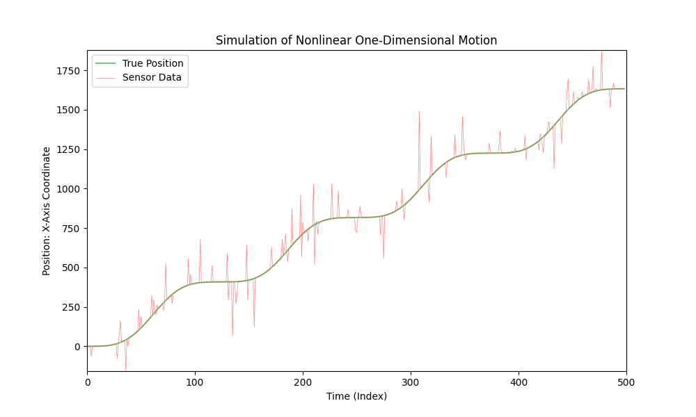
The car moves with varying acceleration, and a sensor measures the car's X-coordinate. In this simulation, we add noise to the sensor data to account for possible measurement errors.

The code provided earlier visualizes this simulation, where the green line represents the "true" position of the car, and the red line represents the sensor data, taking into account the added noise. The acceleration changes over time, creating a more realistic simulation of the car's movement.

This code can be used for visualizing and analyzing different scenarios of car movement, considering changing acceleration and possible sensor errors.

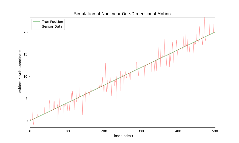
To simulate linear motion, you can simply modify the nonlinear_acceleration(t) function to always return 0:

def nonlinear_acceleration(t):
    return 0

This change will make the car's movement linear with constant velocity.

The Kalman Filter

The Kalman Filter is an algorithm developed by Rudolf E. Kalman in 1960. This algorithm allows for the estimation of the state of a dynamic system based on a set of incomplete and noisy measurements. Initially, the Kalman Filter was developed to address problems in aerospace engineering, but over time, it has found wide applications in various fields. The main advantage of the Kalman Filter is that it is recursive, meaning that it uses the latest measurements and the previous state to compute the current state of the system. This makes it efficient for online real-time data processing.

The Kalman Filter has found applications in many fields, including navigation and vehicle control, signal processing, econometrics, robotics, and many other areas where the estimation of time-varying processes based on imperfect or incomplete data is required.

The Kalman Filter has several key advantages over other data estimation and filtering algorithms:

Optimality: Under certain conditions (linear system, Gaussian noise), the Kalman Filter is optimal in terms of minimizing mean squared estimation error.
Real-time Efficiency: The Kalman Filter is recursive, meaning that it uses only the latest measurements and the previous state to compute the current state. This makes it suitable for real-time applications.
Minimal Memory Requirement: Since the filter only uses the most recent measurement and the current state estimate, it doesn't need to store the entire history of data.
Robustness to Measurement Errors: The filter is capable of efficiently processing noisy data, minimizing the impact of random measurement errors.
Versatile Applications: Due to its versatility, the Kalman Filter has been applied in diverse fields, from aerospace engineering to econometrics.
Ease of Implementation: The algorithm is relatively easy to understand and implement, making it accessible to a wide range of professionals.

Let's implement a basic Kalman Filter for a sensor measuring the position of our car, which is moving in a one-dimensional system with constant velocity but with noisy sensor measurements.

#
#  Copyright (C) 2024, SToFU Systems S.L.
#  All rights reserved.
#
#  This program is free software; you can redistribute it and/or modify
#  it under the terms of the GNU General Public License as published by
#  the Free Software Foundation; either version 3 of the License, or
#  (at your option) any later version.
#
#  This program is distributed in the hope that it will be useful,
#  but WITHOUT ANY WARRANTY; without even the implied warranty of
#  MERCHANTABILITY or FITNESS FOR A PARTICULAR PURPOSE.  See the
#  GNU General Public License for more details.
#
#  You should have received a copy of the GNU General Public License along
#  with this program; if not, write to the Free Software Foundation, Inc.,
#  51 Franklin Street, Fifth Floor, Boston, MA 02110-1301 USA.
#

import matplotlib.pyplot as plt
import numpy as np
from matplotlib.animation import FuncAnimation
from filterpy.kalman import KalmanFilter
from filterpy.common import Q_discrete_white_noise
import sys
import random

# Read noise_percentage, noise_probability, total_points from the command line
noise_percentage = float(sys.argv[1]) / 100.0 if len(sys.argv) > 1 else 0.1
noise_probability = float(sys.argv[2]) / 100.0 if len(sys.argv) > 2 else 0.2
total_points = int(sys.argv[3]) if len(sys.argv) > 3 else 2000
interval = 10 / total_points

# Initialize true positions and velocity
true_positions_linear = [0]
true_velocity = 2

for t in range(1, total_points):
    true_positions_linear.append(true_positions_linear[-1] + true_velocity * interval)

# Function to add noise to true positions
def add_noise(true_positions, probability):
    return [p + np.random.normal(0, scale=noise_percentage * np.mean(true_positions))
            if random.uniform(0, 1) <= probability else p for p in true_positions]

sensor_positions_with_noise = add_noise(true_positions_linear, noise_probability)

# Initialize Kalman Filter (KF)
kf = KalmanFilter(dim_x=2, dim_z=1)
kf.F = np.array([[1, interval],
                 [0, 1]])
kf.H = np.array([[1, 0]])
kf.P *= 1000
kf.R = noise_percentage * np.mean(true_positions_linear)
kf.Q = Q_discrete_white_noise(dim=2, dt=interval, var=0.001)

x = np.array([[sensor_positions_with_noise[0]],
              [0]])
kf_positions = [x[0, 0]]

# Function to update Kalman Filter with sensor data
def update_kalman_filter(z):
    kf.predict()
    kf.update(z)
    return kf.x[0, 0]

# Function to create an animation with Kalman Filter (KF) estimation
def animate_with_kalman(i):
    plt.cla()
    plt.plot(true_positions_linear[:i], color='green', alpha=0.5, label='True Position')
    plt.plot(sensor_positions_with_noise[:i], color='red', alpha=0.5, linewidth=0.5, label='Sensor Data')

    if i < total_points:
        kf_estimate = update_kalman_filter(sensor_positions_with_noise[i])
        kf_positions.append(kf_estimate)

    plt.plot(kf_positions[:i + 1], color='blue', alpha=0.5, label='Kalman Filter (KF) Estimate')

    plt.xlim(0, total_points)
    plt.ylim(min(true_positions_linear + sensor_positions_with_noise),
             max(true_positions_linear + sensor_positions_with_noise))
    plt.xlabel('Time (Index)')
    plt.ylabel('Position: X-Axis Coordinate')
    plt.title('Simulation of Linear One-Dimensional Motion with Kalman Filter (KF)')
    plt.legend()

# Main entry point
if __name__ == "__main__":
    # Create a figure and animation
    fig, ax = plt.subplots(figsize=(10, 6))
    ani = FuncAnimation(fig, animate_with_kalman, frames=total_points, interval=interval * 1000, repeat=False)

    # Display the animation
    plt.show()

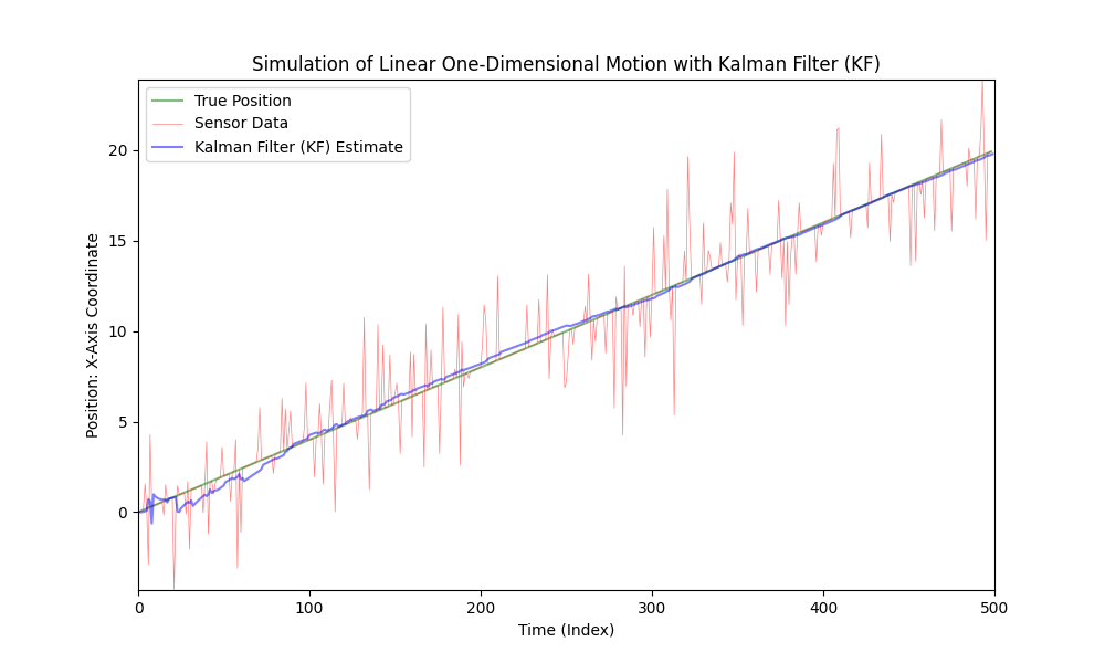
As seen, the Kalman Filter is well-suited for use in linear systems even with strong noise. However, the motion of the car is not linear; the car accelerates with varying magnitudes and directions.

Let's complicate our code a bit by making the car's motion nonlinear and introducing variable acceleration. For simplicity and clarity, we will use a sinusoidal function to model the acceleration. We will keep the noise level the same.

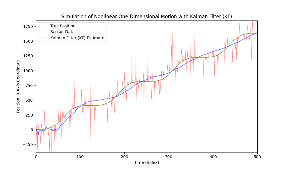
As we can see, the classic Kalman Filter is not suitable for nonlinear models. For these purposes, the Extended Kalman Filter (EKF) was developed.

Extended Kalman Filter (EKF)

The Extended Kalman Filter (EKF) is a modification of the classical Kalman Filter designed to work with nonlinear systems. While the standard Kalman Filter is intended for linear systems, the EKF extends its applicability to handle nonlinear cases.

The Extended Kalman Filter was developed after the original Kalman Filter, introduced by Rudolf Kalman in 1960. It emerged as a result of efforts by engineers and scientists to adapt the Kalman Filter for use with nonlinear systems, especially in the aerospace and marine navigation fields in the 1960s and 1970s. The precise date of its creation and specific authors are less well-known, as the EKF evolved gradually and within the framework of various research groups.

The Extended Kalman Filter (EKF) is widely used in tasks where state estimation of systems described by nonlinear equations is required. Its main application areas include robotics (for estimating the position and orientation of robots), the automotive industry (in autonomous driving systems and navigation), aerospace engineering (for satellite orbital navigation and spacecraft), mobile communications, and many other technical and engineering fields.

The key differences between the Extended Kalman Filter (EKF) and the standard Kalman Filter mainly lie in how they handle the dynamics and measurements of the system.

The primary distinctions include the following:

Handling Nonlinearity: The standard Kalman Filter assumes that the system dynamics and measurement process are linear. This means that the state transition and measurement functions can be represented as linear matrices. The Extended Kalman Filter (EKF) is designed to work with nonlinear systems. Instead of linear matrices, it uses nonlinear functions to describe the system dynamics and measurement process.
Linearization: In the EKF, linearization is used to approximate nonlinear functions, typically through first-order Taylor series expansion around the current state estimate. This provides linearized counterparts of the state transition and measurement functions, which are then used in the filter.
State Transition and Measurement Functions: In the standard Kalman Filter, the state transition and measurement functions are represented by matrices (e.g., state transition matrix and measurement matrix). In the EKF, these functions can be any differentiable nonlinear functions. This adds flexibility but also increases complexity and computational requirements.
Computational Complexity: The EKF requires higher computational complexity due to the need for linearizing nonlinear functions and subsequent calculations.

The main difference between the Extended Kalman Filter and the standard one is its ability to work with nonlinear systems by using nonlinear functions and their linearization.

#
#  Copyright (C) 2024, SToFU Systems S.L.
#  All rights reserved.
#
#  This program is free software; you can redistribute it and/or modify
#  it under the terms of the GNU General Public License as published by
#  the Free Software Foundation; either version 3 of the License, or
#  (at your option) any later version.
#
#  This program is distributed in the hope that it will be useful,
#  but WITHOUT ANY WARRANTY; without even the implied warranty of
#  MERCHANTABILITY or FITNESS FOR A PARTICULAR PURPOSE.  See the
#  GNU General Public License for more details.
#
#  You should have received a copy of the GNU General Public License along
#  with this program; if not, write to the Free Software Foundation, Inc.,
#  51 Franklin Street, Fifth Floor, Boston, MA 02110-1301 USA.
#

import matplotlib.pyplot as plt
import numpy as np
from matplotlib.animation import FuncAnimation
from filterpy.kalman import KalmanFilter
from filterpy.common import Q_discrete_white_noise
import sys
import random

# Named constants
AMPLITUDE_FACTOR = 5.0  # Factor for amplitude in the nonlinear acceleration function
WAVES = 4  # Number of waves in the nonlinear motion model
INITIAL_POSITION = 0  # Initial position
TRUE_VELOCITY_INITIAL = 2.0  # Initial true velocity (changed to float)
TRUE_VELOCITY_INCREMENT = 0.2  # Increment for true velocity (added as a constant)
PREDICTION_INTERVAL = 10  # Interval for predictions
DIM_X = 2  # Dimension of state vector in Kalman filter
DIM_Z = 1  # Dimension of measurement vector in Kalman filter
INITIAL_P_COVARIANCE = 1000  # Initial state covariance for Kalman filter

# Initialize random number generator with the current time
random.seed()

# Read noise_percentage, noise_probability, and total_points from command line arguments
noise_percentage = float(sys.argv[1]) / 100.0 if len(sys.argv) > 1 else 0.1
noise_probability = float(sys.argv[2]) / 100.0 if len(sys.argv) > 2 else 0.2
total_points = int(sys.argv[3]) if len(sys.argv) > 3 else 2000
interval = PREDICTION_INTERVAL / total_points  # Time interval between data points

# Define a nonlinear acceleration function that varies with time
def nonlinear_acceleration(t):
    # Calculate the amplitude of acceleration based on time
    amplitude = AMPLITUDE_FACTOR * 200.0 * (1 - abs((t % (total_points / WAVES) - (total_points / (2 * WAVES))) / (total_points / (2 * WAVES))))
    # Calculate the nonlinear acceleration based on time and amplitude
    return amplitude * np.sin(2.0 * np.pi * t / (total_points / WAVES))

# Function to add noise to true positions with a given probability
def add_noise(true_positions, probability):
    # Add Gaussian noise to true positions with specified probability
    return [p + np.random.normal(0, scale=noise_percentage * np.mean(true_positions)) if random.uniform(0, 1) <= probability else p for p in true_positions]

# Function to update the Extended Kalman Filter (EKF) with sensor measurements
def update_extended_kalman_filter(z):
    ekf.predict()  # Predict the next state
    ekf.update(z)  # Update the state based on sensor measurements
    return ekf.x[0, 0]  # Return the estimated position

# Функция для закрытия анимации при нажатии клавиши ESC
def close_animation(event):
    if event.key == 'escape':
        plt.close()

# Function for creating an animation with EKF estimates
def animate_with_ekf(i):
    plt.cla()
    # Plot the true position and sensor data up to the current time
    plt.plot(true_positions_nonlinear[:i], color='green', alpha=0.5, label='True Position')
    plt.plot(sensor_positions_with_noise[:i], color='red', alpha=0.5, label='Sensor Data', linewidth=0.5)

    if i < total_points:
        # Update the EKF with the current sensor measurement and obtain the estimate
        ekf_estimate = update_extended_kalman_filter(sensor_positions_with_noise[i])
        ekf_positions.append(ekf_estimate)

    # Plot the EKF estimate up to the current time
    plt.plot(ekf_positions[:i + 1], color='purple', alpha=0.5, label='Extended Kalman Filter (EKF) Estimate')

    # Set plot limits and labels
    plt.xlim(0, total_points)
    plt.ylim(min(true_positions_nonlinear + sensor_positions_with_noise),
             max(true_positions_nonlinear + sensor_positions_with_noise))
    plt.xlabel('Time (Index)')
    plt.ylabel('Position: X-Axis Coordinate')
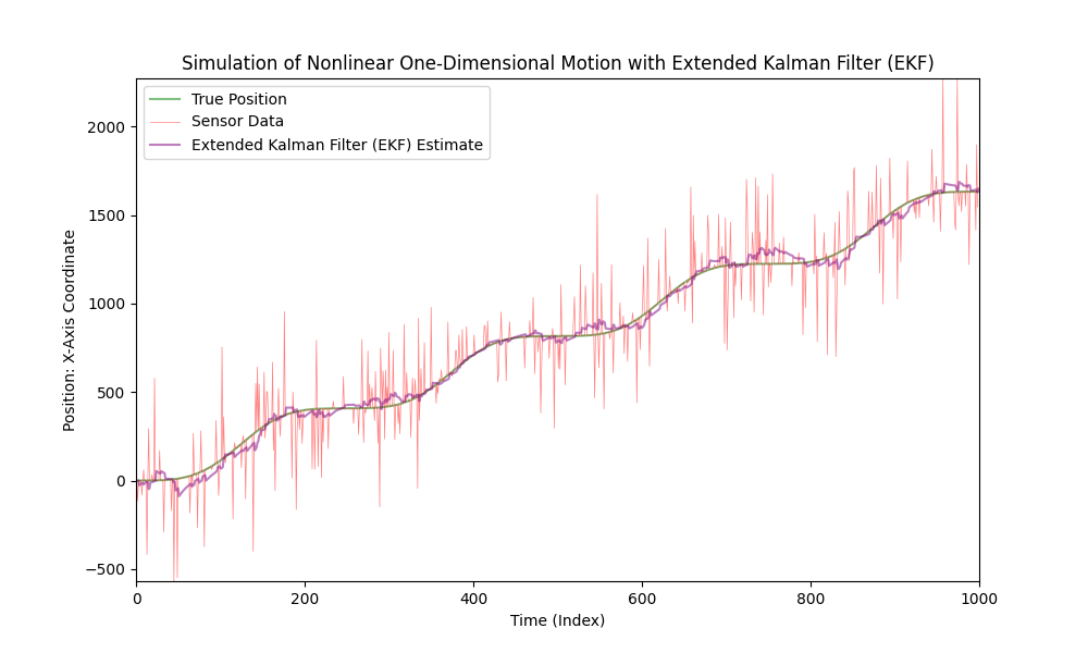
    plt.title('Simulation of Nonlinear One-Dimensional Motion with Extended Kalman Filter (EKF)')
    plt.legend()

# Main entry point of the code
if __name__ == "__main__":
    # Create a figure for the animation
    fig, ax = plt.subplots(figsize=(10, 6))

    # Используйте connect для добавления обработчика событий
    fig.canvas.mpl_connect('key_press_event', close_animation)

    # Initialize true_positions_nonlinear with the initial position and true_velocity
    true_positions_nonlinear = [INITIAL_POSITION]
    true_velocity = TRUE_VELOCITY_INITIAL

    # Generate true positions based on the nonlinear motion model
    for t in range(1, total_points):
        acc = nonlinear_acceleration(t)
        true_velocity += acc * interval
        true_positions_nonlinear.append(true_positions_nonlinear[-1] + true_velocity * interval)

    # Add noise to true positions to simulate sensor data
    sensor_positions_with_noise = add_noise(true_positions_nonlinear, noise_probability)

    # Initialize an Extended Kalman Filter (EKF)
    ekf = KalmanFilter(dim_x=DIM_X, dim_z=DIM_Z)
    ekf.F = np.array([[1, interval],
                    [0, 1]])
    ekf.H = np.array([[1, 0]])
    ekf.P *= INITIAL_P_COVARIANCE
    ekf.R = noise_percentage * np.mean(true_positions_nonlinear)

    ekf_x = np.array([[sensor_positions_with_noise[0]],
                    [0]])
    ekf_positions = [ekf_x[0, 0]]

    # Create the animation using FuncAnimation
    ani = FuncAnimation(fig, animate_with_ekf, frames=total_points, interval=interval * 1000, repeat=False)

    # Display the animation
    plt.show()

Apply the Extended Kalman Filter for nonlinear motion.

Now, let's significantly increase the level of sensor noise.

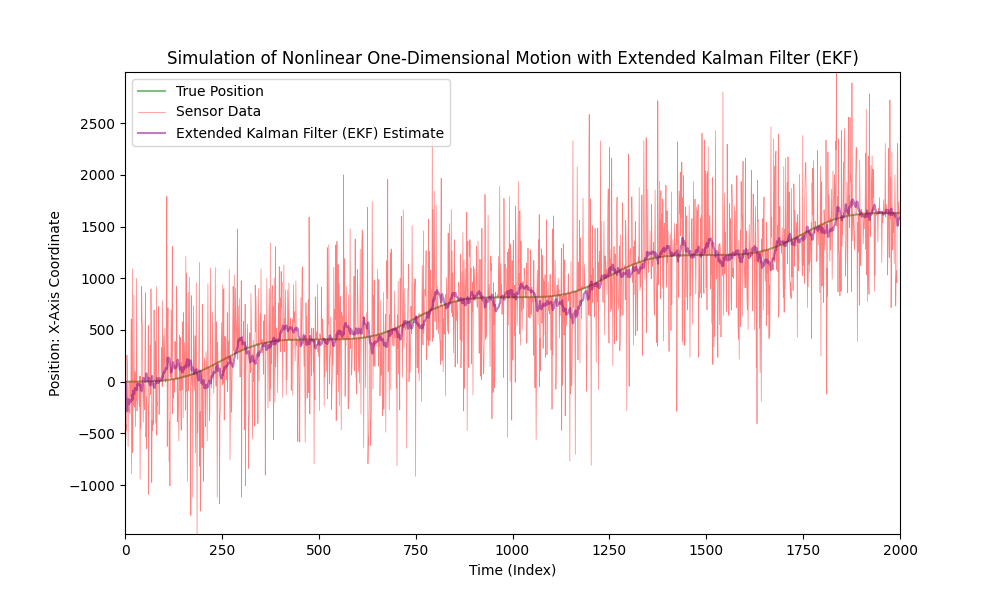
As we can see, the Extended Kalman Filter performs well even in cases of highly noisy data.

Additional materials

https://en.wikipedia.org/wiki/Kalman_filter - Description of the filter and its fundamental mathematical principles of operation.

https://kalmanfilter.org/cpp/index.html - Description and implementation of the filter in C++.

https://commons.apache.org/proper/commons-math/javadocs/api-3.6.1/org/apache/commons/math3/filter/KalmanFilter.html - Description and implementation of the filter in Java.

https://filterpy.readthedocs.io/en/latest/kalman/KalmanFilter.html - Description and implementation of the filter in Python

Conclusion

The Extended Kalman Filter (EKF) is a powerful tool for estimating the state of dynamic systems, especially when this estimation needs to be based on data from multiple sensors simultaneously. One of the key advantages of the EKF is its ability to integrate information from various sources, making it exceptionally useful in complex systems such as automotive navigation systems, robotics, or aerospace engineering.

Considering noisy and often imperfect data from different sensors, the EKF is capable of merging this data into a unified whole, providing a more accurate and reliable state estimate. For example, in a car, the EKF can use GPS data to determine position and accelerometer data to calculate speed and acceleration, thereby creating a more complete picture of the vehicle's motion.

The Extended Kalman Filter (EKF) is capable of reducing the overall uncertainty arising from the noise and errors of each individual sensor. Since these errors are often uncorrelated, their joint processing in the EKF enables more stable and accurate estimates. It is also worth noting that the EKF exhibits high robustness: in case of problems with one of the sensors, the system can continue to operate relying on data from the remaining ones. This makes the EKF particularly valuable in critical applications where reliability and accuracy are of paramount importance. Another important aspect when working with multiple sensors is the time synchronization of measurements. The EKF adeptly handles these temporal differences, ensuring correct data fusion.

Thanks to its ability to aggregate and analyze information from multiple sources, the EKF is an invaluable tool in areas where high precision state estimation is required under conditions of uncertainty and dynamic changes.

In conclusion, software combating sensor noise is a challenging process that encompasses static, statistical methods and the application of artificial intelligence for noise type classification and mitigation.

Our company possesses substantial expertise in dealing with sensor noise issues.

For inquiries regarding this article, please feel free to contact us at articles@stofu.io.

For collaboration opportunities, you can reach out to us at info@stofu.io.

All code files you can find in our repository: https://github.com/SToFU-Systems/EKF_Usage.

Wishing you all the best,

SToFU Systems Team

https://stofu.io

Software Approach to Dealing with ADAS Sensor Noise (Part 1)

What is ADAS?

Sensor Noise in ADAS

Simulation of Point Movement in a One-Dimensional Coordinate System

The Kalman Filter

Extended Kalman Filter (EKF)

Additional materials

Conclusion

Categories

Recent Posts

Software Approach to Dealing with ADAS Sensor Noise (Part 1)

PE Resource Parser in C++ (Native)

Introduction to Windows Kernel Development on Rust (PaRT 1)

Introduction to a GPU programming

Inside BlackMatter: Technical Analysis of BlackMatter Ransomware