ADAS 센서 노이즈 처리를 위한 소프트웨어 접근 (1부)

ADAS란 무엇인가?

현대 자동차는 ADAS (Advanced Driver Assistance Systems) 덕분에 점점 더 스마트해지고 있습니다. 이 시스템들은 도로 안전을 향상시키고 운전을 더 편안하게 만들어줍니다. 카메라, 레이더 및 기타 센서를 사용하는 이 시스템들은 차량 제어를 돕고, 다른 차량, 보행자, 교통 신호등을 감지하며, 도로 상태와 주변 환경에 대한 최신 정보를 운전자에게 제공합니다.

ADAS는 앞차의 속도에 맞춰 자동차의 속도를 조절하는 적응형 크루즈 컨트롤, 차선 유지 시스템을 통해 차량이 차선 내에 있도록 하는 기능, 충돌 방지를 위한 자동 제동, 주차 동작을 용이하게 하는 자동 주차 시스템과 같은 다양한 기능을 포함합니다. 카메라, 레이더, 라이다, 초음파 센서와 같은 다양한 유형의 센서가 이러한 시스템의 기능을 보장하며, 차량이 도로 상황 및 운전자의 운전 스타일에 적응할 수 있도록 돕습니다.

ADAS에서의 센서 노이즈

ADAS 센서는 현대적이고 복잡함에도 불구하고 잡음 간섭에 취약합니다. 이는 여러 이유로 발생합니다. 우선, 환경이 센서에 예측할 수 없는 영향을 줄 수 있습니다. 예를 들어, 먼지, 진흙, 비, 또는 눈이 카메라와 레이더를 덮어 정보 수신을 왜곡할 수 있습니다. 이는 더러운 유리를 통해 바라보는 것과 같습니다: 모든 것이 보이지 않고 명확하지 않으며, 많은 잡티에 의해 시야가 가려집니다. 둘째, 센서 자체의 기술적 한계도 잡음을 유발할 수 있습니다. 예를 들어, 센서는 저조도 환경이나 강한 빛 대비에서 성능이 떨어질 수 있습니다. 이는 어둠 속에서 무언가를 식별하려 하거나 지나치게 밝은 빛원을 바라보는 것과 비슷합니다 - 두 경우 모두 세부 사항을 보는 것이 극도로 어려워집니다. 센서에서 받은 데이터가 왜곡되면, 운전 보조 시스템이 도로 상황을 잘못 해석할 수 있으며, 이는 특정 상황에서 교통사고 위험을 증가시킬 수 있습니다.

일차원 좌표 시스템에서의 점 움직임 시뮬레이션

먼저, 일차원 공간에서 자동차의 움직임을 시뮬레이션하는 코드를 작성해보겠습니다. 코드를 실행하기 위해서는 Python 환경을 구축하고 필요한 라이브러리를 설치해야 합니다.

라이브러리를 설치하고 코드를 실행하는 단계는 다음과 같습니다:

코드를 실행하려면 Python 환경을 설정하고 필요한 라이브러리를 설치해야 합니다. 라이브러리 설치 및 코드 실행을 위한 단계는 다음과 같습니다: Python 설치: 아직 Python이 없다면 공식 Python 웹사이트(https://www.python.org/downloads/)에서 다운로드하여 설치하세요. Python 버전 3.x 사용을 권장합니다.
필요한 라이브러리 설치: 명령 줄을 열고(Windows에서는 명령 프롬프트 또는 PowerShell일 수 있습니다) 다음 명령을 실행하여 라이브러리를 설치합니다:
```
pip install matplotlib numpy filterpy
```
코드 저장: 제공한 코드를 복사하여 .py 확장자를 가진 파일에 저장하세요(예: simulation.py)
코드 실행: 명령 줄에서 코드 파일이 위치한 디렉토리로 이동하여 다음 명령으로 실행하세요:
```
python simulation.py 20 20 500
```
이 명령은 노이즈 진폭(20), 노이즈 주파수(20), 그래프의 총 데이터 포인트 수(500)에 대한 인수를 사용하여 코드를 실행합니다. 필요에 따라 인수 값을 변경할 수 있습니다.

#
#  Copyright (C) 2024, SToFU Systems S.L.
#  All rights reserved.
#
#  This program is free software; you can redistribute it and/or modify
#  it under the terms of the GNU General Public License as published by
#  the Free Software Foundation; either version 3 of the License, or
#  (at your option) any later version.
#
#  This program is distributed in the hope that it will be useful,
#  but WITHOUT ANY WARRANTY; without even the implied warranty of
#  MERCHANTABILITY or FITNESS FOR A PARTICULAR PURPOSE.  See the
#  GNU General Public License for more details.
#
#  You should have received a copy of the GNU General Public License along
#  with this program; if not, write to the Free Software Foundation, Inc.,
#  51 Franklin Street, Fifth Floor, Boston, MA 02110-1301 USA.
#

import matplotlib.pyplot as plt
import numpy as np
from matplotlib.animation import FuncAnimation
import sys
import random
import time

# Named constants
AMPLITUDE_FACTOR = 5.0  # Factor for amplitude in the nonlinear acceleration function
WAVES = 4  # Number of waves in the nonlinear motion model
INITIAL_POSITION = 0  # Initial position
TRUE_VELOCITY_INITIAL = 2.0  # Initial true velocity (changed to float)
TRUE_VELOCITY_INCREMENT = 0.2  # Increment for true velocity (added as a constant)
PREDICTION_INTERVAL = 10  # Interval for predictions
DIM_X = 2  # Dimension of state vector in Kalman filter
DIM_Z = 1  # Dimension of measurement vector in Kalman filter
INITIAL_P_COVARIANCE = 1000  # Initial state covariance for Kalman filter
RANDOM_SEED = 42  # Seed for random number generator

# Initialize random number generator with the current time
random.seed(int(time.time()))  # Using the current time to initialize the random number generator

# Read noise_percentage, noise_probability, and total_points from command line arguments
noise_percentage = float(sys.argv[1]) / 100.0 if len(sys.argv) > 1 else 0.1
noise_probability = float(sys.argv[2]) / 100.0 if len(sys.argv) > 2 else 0.2
total_points = int(sys.argv[3]) if len(sys.argv) > 3 else 2000
interval = PREDICTION_INTERVAL / total_points  # Time interval between data points

# Define a nonlinear acceleration function that varies with time
def nonlinear_acceleration(t):
    # Calculate the amplitude of acceleration based on time
    amplitude = AMPLITUDE_FACTOR * 200.0 * (1 - abs((t % (total_points / WAVES) - (total_points / (2 * WAVES))) / (total_points / (2 * WAVES))))
    # Calculate the nonlinear acceleration based on time and amplitude
    return amplitude * np.sin(2.0 * np.pi * t / (total_points / WAVES))

# Function to add noise to true positions with a given probability
def add_noise(true_positions, probability):
    # Add Gaussian noise to true positions with specified probability
    return [p + np.random.normal(0, scale=noise_percentage * np.mean(true_positions)) if random.uniform(0, 1) <= probability else p for p in true_positions]

# Function to close the animation on pressing the ESC key
def close_animation(event):
    if event.key == 'escape':
        plt.close()

# Function for creating an animation without the Kalman Filter
def animate_without_ekf(i):
    plt.cla()
    # Plot the true position and sensor data up to the current time
    plt.plot(true_positions_nonlinear[:i], color='green', alpha=0.5, label='True Position')
    plt.plot(sensor_positions_with_noise[:i], color='red', alpha=0.5, label='Sensor Data', linewidth=0.5)

    # Set plot limits and labels
    plt.xlim(0, total_points)
    plt.ylim(min(true_positions_nonlinear + sensor_positions_with_noise),
             max(true_positions_nonlinear + sensor_positions_with_noise))
    plt.xlabel('Time (Index)')
    plt.ylabel('Position: X-Axis Coordinate')
    plt.title('Simulation of Nonlinear One-Dimensional Motion')

    # Display the legend
    plt.legend()

# Main entry point of the code
if __name__ == "__main__":
    # Create a figure for the animation
    fig, ax = plt.subplots(figsize=(10, 6))

    # Use connect to add an event handler for key presses
    fig.canvas.mpl_connect('key_press_event', close_animation)

    # Initialize true_positions_nonlinear with the initial position and true_velocity
    true_positions_nonlinear = [INITIAL_POSITION]
    true_velocity = TRUE_VELOCITY_INITIAL

    # Generate true positions based on the nonlinear motion model
    for t in range(1, total_points):
        acc = nonlinear_acceleration(t)
        true_velocity += acc * interval
        true_positions_nonlinear.append(true_positions_nonlinear[-1] + true_velocity * interval)

    # Add noise to true positions to simulate sensor data
    sensor_positions_with_noise = add_noise(true_positions_nonlinear, noise_probability)

    # Create the animation using FuncAnimation
    ani = FuncAnimation(fig, animate_without_ekf, frames=total_points, interval=interval * 1000, repeat=False)

    # Display the animation
    plt.show()

이것은 일차원 공간에서 자동차의 움직임을 시뮬레이션한 것입니다:

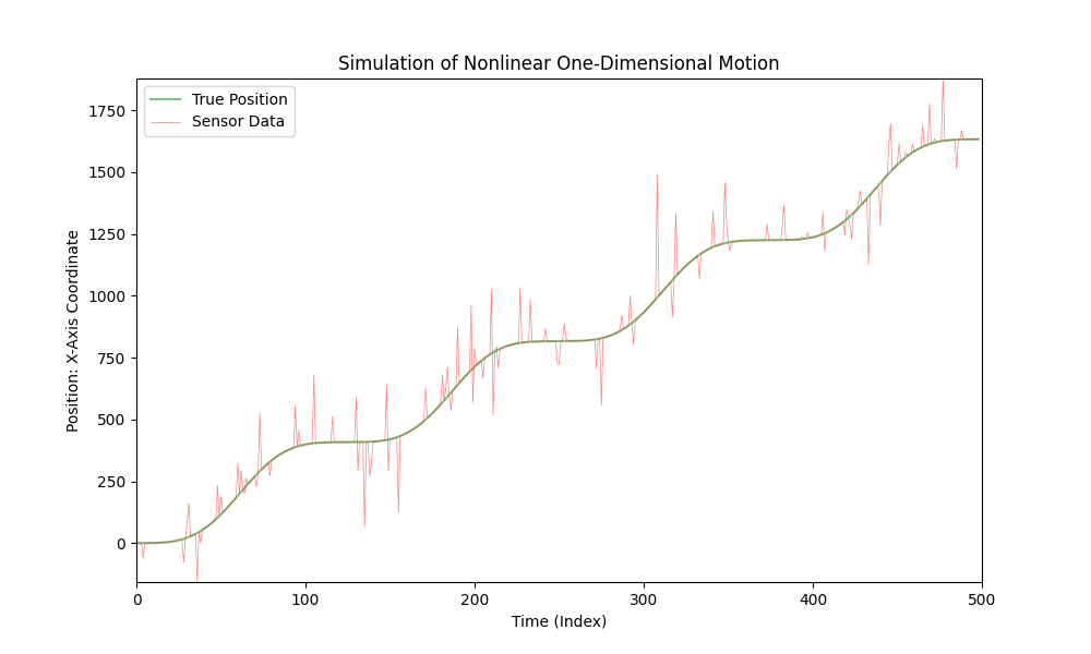
자동차는 다양한 가속도로 움직이며, 센서가 자동차의 X좌표를 측정합니다. 이 시뮬레이션에서는 가능한 측정 오류를 고려하여 센서 데이터에 잡음을 추가합니다.

앞서 제공된 코드는 이 시뮬레이션을 시각화합니다. 여기서 초록색 선은 자동차의 "진짜" 위치를 나타내고, 빨간색 선은 추가된 잡음을 고려한 센서 데이터를 나타냅니다. 가속도가 시간에 따라 변화하여 자동차의 움직임을 더 현실적으로 시뮬레이션합니다.

이 코드는 가속도 변화와 가능한 센서 오류를 고려하여 자동차 움직임의 다양한 시나리오를 시각화하고 분석하는 데 사용할 수 있습니다.

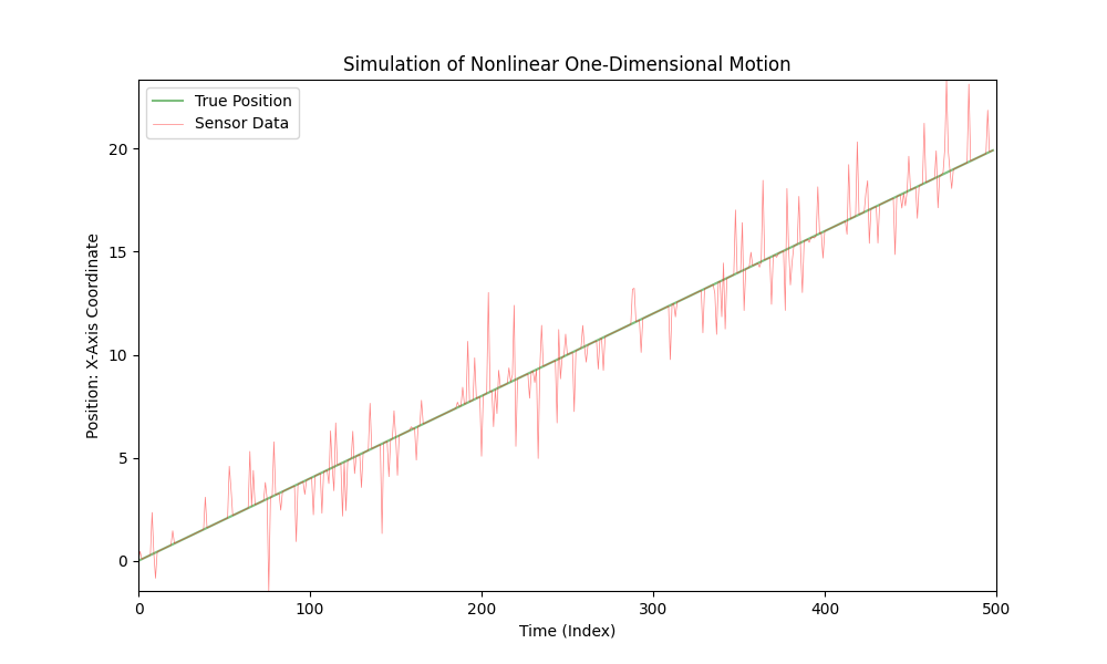
선형 운동을 모의하려면, nonlinear_acceleration(t) 함수를 항상 0을 반환하도록 수정하면 됩니다:

def nonlinear_acceleration(t):
    return 0

이 변경으로 자동차의 운동이 일정한 속도로 선형적이 될 것입니다.

칼만 필터

Kalman Filter는 1960년에 Rudolf E. Kalman이 개발한 알고리즘입니다. 이 알고리즘은 불완전하고 잡음이 섞인 측정치들을 바탕으로 동적 시스템의 상태를 추정할 수 있게 합니다. 처음에 Kalman Filter는 항공우주 공학의 문제를 해결하기 위해 개발되었지만, 시간이 지남에 따라 다양한 분야에서 널리 활용되고 있습니다. Kalman Filter의 주요 장점은 재귀적이라는 것인데, 이는 가장 최신의 측정치와 이전 상태를 사용하여 시스템의 현재 상태를 계산한다는 의미입니다. 이로 인해 온라인 실시간 데이터 처리에 효율적입니다.

Kalman 필터는 항법 및 차량 제어, 신호 처리, 계량경제학, 로보틱스 및 불완전하거나 불완전한 데이터를 기반으로 시간 변화 과정을 추정해야 하는 많은 다른 분야에서 응용을 찾았습니다.

Kalman Filter는 다른 데이터 추정 및 필터링 알고리즘에 비해 여러 가지 중요한 장점을 가지고 있습니다:

최적성: 특정 조건(선형 시스템, 가우스 잡음) 하에서, 칼만 필터는 평균 제곱 추정 오류를 최소화하는 측면에서 최적입니다.
실시간 효율성: 칼만 필터는 재귀적이며, 이는 가장 최근의 측정값과 이전 상태만을 사용하여 현재 상태를 계산한다는 의미입니다. 이로 인해 실시간 응용 프로그램에 적합합니다.
최소 메모리 요구 사항: 필터는 가장 최근의 측정값과 현재 상태 추정치만을 사용하기 때문에, 전체 데이터의 역사를 저장할 필요가 없습니다.
측정 오류에 대한 강건성: 필터는 잡음이 많은 데이터를 효율적으로 처리할 수 있으며, 임의의 측정 오류의 영향을 최소화합니다.
다양한 응용: 그 다재다능함으로 인해, 칼만 필터는 항공우주 공학부터 계량 경제학에 이르기까지 다양한 분야에 적용되었습니다.
구현 용이성: 알고리즘은 비교적 이해하고 구현하기 쉬워, 다양한 전문가들에게 접근성이 좋습니다.

우리의 자동차의 위치를 측정하는 센서를 위한 기본 칼만 필터를 구현해 봅시다. 이 자동차는 일정한 속도로 움직이는 일차원 시스템에서 운행되지만 센서 측정에는 노이즈가 있습니다.

#
#  Copyright (C) 2024, SToFU Systems S.L.
#  All rights reserved.
#
#  This program is free software; you can redistribute it and/or modify
#  it under the terms of the GNU General Public License as published by
#  the Free Software Foundation; either version 3 of the License, or
#  (at your option) any later version.
#
#  This program is distributed in the hope that it will be useful,
#  but WITHOUT ANY WARRANTY; without even the implied warranty of
#  MERCHANTABILITY or FITNESS FOR A PARTICULAR PURPOSE.  See the
#  GNU General Public License for more details.
#
#  You should have received a copy of the GNU General Public License along
#  with this program; if not, write to the Free Software Foundation, Inc.,
#  51 Franklin Street, Fifth Floor, Boston, MA 02110-1301 USA.
#

import matplotlib.pyplot as plt
import numpy as np
from matplotlib.animation import FuncAnimation
from filterpy.kalman import KalmanFilter
from filterpy.common import Q_discrete_white_noise
import sys
import random

# Read noise_percentage, noise_probability, total_points from the command line
noise_percentage = float(sys.argv[1]) / 100.0 if len(sys.argv) > 1 else 0.1
noise_probability = float(sys.argv[2]) / 100.0 if len(sys.argv) > 2 else 0.2
total_points = int(sys.argv[3]) if len(sys.argv) > 3 else 2000
interval = 10 / total_points

# Initialize true positions and velocity
true_positions_linear = [0]
true_velocity = 2

for t in range(1, total_points):
    true_positions_linear.append(true_positions_linear[-1] + true_velocity * interval)

# Function to add noise to true positions
def add_noise(true_positions, probability):
    return [p + np.random.normal(0, scale=noise_percentage * np.mean(true_positions))
            if random.uniform(0, 1) <= probability else p for p in true_positions]

sensor_positions_with_noise = add_noise(true_positions_linear, noise_probability)

# Initialize Kalman Filter (KF)
kf = KalmanFilter(dim_x=2, dim_z=1)
kf.F = np.array([[1, interval],
                 [0, 1]])
kf.H = np.array([[1, 0]])
kf.P *= 1000
kf.R = noise_percentage * np.mean(true_positions_linear)
kf.Q = Q_discrete_white_noise(dim=2, dt=interval, var=0.001)

x = np.array([[sensor_positions_with_noise[0]],
              [0]])
kf_positions = [x[0, 0]]

# Function to update Kalman Filter with sensor data
def update_kalman_filter(z):
    kf.predict()
    kf.update(z)
    return kf.x[0, 0]

# Function to create an animation with Kalman Filter (KF) estimation
def animate_with_kalman(i):
    plt.cla()
    plt.plot(true_positions_linear[:i], color='green', alpha=0.5, label='True Position')
    plt.plot(sensor_positions_with_noise[:i], color='red', alpha=0.5, linewidth=0.5, label='Sensor Data')

    if i < total_points:
        kf_estimate = update_kalman_filter(sensor_positions_with_noise[i])
        kf_positions.append(kf_estimate)

    plt.plot(kf_positions[:i + 1], color='blue', alpha=0.5, label='Kalman Filter (KF) Estimate')

    plt.xlim(0, total_points)
    plt.ylim(min(true_positions_linear + sensor_positions_with_noise),
             max(true_positions_linear + sensor_positions_with_noise))
    plt.xlabel('Time (Index)')
    plt.ylabel('Position: X-Axis Coordinate')
    plt.title('Simulation of Linear One-Dimensional Motion with Kalman Filter (KF)')
    plt.legend()

# Main entry point
if __name__ == "__main__":
    # Create a figure and animation
    fig, ax = plt.subplots(figsize=(10, 6))
    ani = FuncAnimation(fig, animate_with_kalman, frames=total_points, interval=interval * 1000, repeat=False)

    # Display the animation
    plt.show()

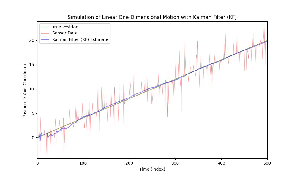
Kalman Filter는 강한 잡음이 있어도 선형 시스템에서 사용하기에 적합한 것으로 나타났습니다. 그러나 자동차의 움직임은 선형이 아니며, 자동차는 다양한 크기와 방향으로 가속합니다.

코드를 좀 더 복잡하게 하기 위해 차의 움직임을 비선형으로 만들고 가변 가속도를 도입하겠습니다. 단순성과 명확성을 위해, 가속도를 모델링하기 위해 사인 함수를 사용하겠습니다. 소음 수준은 동일하게 유지하겠습니다.

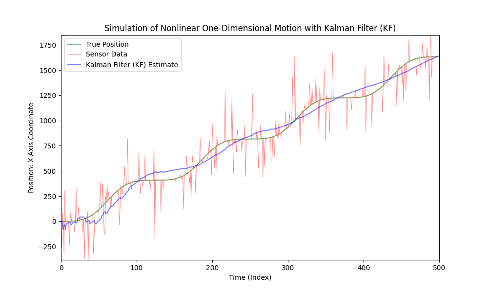
우리가 볼 수 있듯이, 클래식 칼만 필터는 비선형 모델에 적합하지 않습니다. 이러한 목적을 위해 Extended Kalman Filter (EKF)가 개발되었습니다.

확장 칼만 필터 (Extended Kalman Filter, EKF)

확장 칼만 필터(Extended Kalman Filter, EKF)는 비선형 시스템에서 작동하도록 고안된 고전적인 칼만 필터의 수정 버전입니다. 표준 칼만 필터가 선형 시스템을 위한 것인 반면, EKF는 비선형 경우를 처리할 수 있도록 그 적용 범위를 확장합니다.

확장 칼만 필터(Extended Kalman Filter)는 1960년 루돌프 칼만(Rudolf Kalman)에 의해 도입된 원래의 칼만 필터(Kalman Filter) 이후 개발되었습니다. 이는 1960년대와 1970년대 항공우주 및 해양 항법 분야에서 비선형 시스템에 칼만 필터를 적용하기 위한 엔지니어와 과학자들의 노력의 결과로 등장했습니다. 그 창조의 정확한 날짜와 구체적인 저자들은 잘 알려져 있지 않으며, EKF는 점차적으로 여러 연구 그룹의 틀 내에서 진화했습니다.

확장 칼만 필터(Extended Kalman Filter, EKF)는 비선형 방정식으로 기술된 시스템의 상태 추정이 필요한 작업에서 널리 사용됩니다. 주요 응용 분야로는 로보틱스(로봇의 위치와 방향 추정을 위해), 자동차 산업(자율 주행 시스템 및 내비게이션에서), 항공우주 공학(위성 궤도 내비게이션 및 우주선을 위해), 이동 통신 등 많은 기술 및 공학 분야가 있습니다.

확장 칼만 필터(Extended Kalman Filter, EKF)와 표준 칼만 필터와의 주요 차이점은 시스템의 동역학과 측정을 처리하는 방식에 주로 있습니다.

주요 차이점은 다음과 같습니다:

비선형 처리: 표준 칼만 필터는 시스템 동역학과 측정 과정이 선형이라고 가정합니다. 이는 상태 전이와 측정 함수가 선형 행렬로 표현될 수 있다는 의미입니다. Extended Kalman Filter (EKF)는 비선형 시스템으로 작동하도록 설계되었습니다. 선형 행렬 대신, 시스템 동역학과 측정 과정을 설명하기 위해 비선형 함수를 사용합니다.
선형화: EKF에서는 비선형 함수를 근사하기 위해 선형화가 사용되며, 일반적으로 현재 상태 추정 주변의 일차 테일러 급수 확장을 통해 이루어집니다. 이로써 상태 전이와 측정 함수의 선형화된 대응물이 제공되며, 필터에서 사용됩니다.
상태 전이 및 측정 함수: 표준 칼만 필터에서는 상태 전이와 측정 함수가 행렬(예: 상태 전이 행렬 및 측정 행렬)로 나타납니다. EKF에서는 이러한 함수가 어떠한 미분 가능한 비선형 함수가 될 수 있습니다. 이는 유연성을 추가하지만 복잡성과 계산 요구 사항도 증가시킵니다.
계산 복잡성: EKF는 비선형 함수를 선형화하고 그에 따른 계산을 필요로 하기 때문에 더 높은 계산 복잡성을 요구합니다.

확장 칼만 필터와 표준 필터의 주요 차이점은 비선형 시스템에서도 작동할 수 있도록 비선형 함수와 그 선형화를 사용하는 능력에 있습니다.

#
#  Copyright (C) 2024, SToFU Systems S.L.
#  All rights reserved.
#
#  This program is free software; you can redistribute it and/or modify
#  it under the terms of the GNU General Public License as published by
#  the Free Software Foundation; either version 3 of the License, or
#  (at your option) any later version.
#
#  This program is distributed in the hope that it will be useful,
#  but WITHOUT ANY WARRANTY; without even the implied warranty of
#  MERCHANTABILITY or FITNESS FOR A PARTICULAR PURPOSE.  See the
#  GNU General Public License for more details.
#
#  You should have received a copy of the GNU General Public License along
#  with this program; if not, write to the Free Software Foundation, Inc.,
#  51 Franklin Street, Fifth Floor, Boston, MA 02110-1301 USA.
#

import matplotlib.pyplot as plt
import numpy as np
from matplotlib.animation import FuncAnimation
from filterpy.kalman import KalmanFilter
from filterpy.common import Q_discrete_white_noise
import sys
import random

# Named constants
AMPLITUDE_FACTOR = 5.0  # Factor for amplitude in the nonlinear acceleration function
WAVES = 4  # Number of waves in the nonlinear motion model
INITIAL_POSITION = 0  # Initial position
TRUE_VELOCITY_INITIAL = 2.0  # Initial true velocity (changed to float)
TRUE_VELOCITY_INCREMENT = 0.2  # Increment for true velocity (added as a constant)
PREDICTION_INTERVAL = 10  # Interval for predictions
DIM_X = 2  # Dimension of state vector in Kalman filter
DIM_Z = 1  # Dimension of measurement vector in Kalman filter
INITIAL_P_COVARIANCE = 1000  # Initial state covariance for Kalman filter

# Initialize random number generator with the current time
random.seed()

# Read noise_percentage, noise_probability, and total_points from command line arguments
noise_percentage = float(sys.argv[1]) / 100.0 if len(sys.argv) > 1 else 0.1
noise_probability = float(sys.argv[2]) / 100.0 if len(sys.argv) > 2 else 0.2
total_points = int(sys.argv[3]) if len(sys.argv) > 3 else 2000
interval = PREDICTION_INTERVAL / total_points  # Time interval between data points

# Define a nonlinear acceleration function that varies with time
def nonlinear_acceleration(t):
    # Calculate the amplitude of acceleration based on time
    amplitude = AMPLITUDE_FACTOR * 200.0 * (1 - abs((t % (total_points / WAVES) - (total_points / (2 * WAVES))) / (total_points / (2 * WAVES))))
    # Calculate the nonlinear acceleration based on time and amplitude
    return amplitude * np.sin(2.0 * np.pi * t / (total_points / WAVES))

# Function to add noise to true positions with a given probability
def add_noise(true_positions, probability):
    # Add Gaussian noise to true positions with specified probability
    return [p + np.random.normal(0, scale=noise_percentage * np.mean(true_positions)) if random.uniform(0, 1) <= probability else p for p in true_positions]

# Function to update the Extended Kalman Filter (EKF) with sensor measurements
def update_extended_kalman_filter(z):
    ekf.predict()  # Predict the next state
    ekf.update(z)  # Update the state based on sensor measurements
    return ekf.x[0, 0]  # Return the estimated position

# Функция для закрытия анимации при нажатии клавиши ESC
def close_animation(event):
    if event.key == 'escape':
        plt.close()

# Function for creating an animation with EKF estimates
def animate_with_ekf(i):
    plt.cla()
    # Plot the true position and sensor data up to the current time
    plt.plot(true_positions_nonlinear[:i], color='green', alpha=0.5, label='True Position')
    plt.plot(sensor_positions_with_noise[:i], color='red', alpha=0.5, label='Sensor Data', linewidth=0.5)

    if i < total_points:
        # Update the EKF with the current sensor measurement and obtain the estimate
        ekf_estimate = update_extended_kalman_filter(sensor_positions_with_noise[i])
        ekf_positions.append(ekf_estimate)

    # Plot the EKF estimate up to the current time
    plt.plot(ekf_positions[:i + 1], color='purple', alpha=0.5, label='Extended Kalman Filter (EKF) Estimate')

    # Set plot limits and labels
    plt.xlim(0, total_points)
    plt.ylim(min(true_positions_nonlinear + sensor_positions_with_noise),
             max(true_positions_nonlinear + sensor_positions_with_noise))
    plt.xlabel('Time (Index)')
    plt.ylabel('Position: X-Axis Coordinate')
    plt.title('Simulation of Nonlinear One-Dimensional Motion with Extended Kalman Filter (EKF)')
    plt.legend()

# Main entry point of the code
if __name__ == "__main__":
    # Create a figure for the animation
    fig, ax = plt.subplots(figsize=(10, 6))

    # Используйте connect для добавления обработчика событий
    fig.canvas.mpl_connect('key_press_event', close_animation)

    # Initialize true_positions_nonlinear with the initial position and true_velocity
    true_positions_nonlinear = [INITIAL_POSITION]
    true_velocity = TRUE_VELOCITY_INITIAL

    # Generate true positions based on the nonlinear motion model
    for t in range(1, total_points):
        acc = nonlinear_acceleration(t)
        true_velocity += acc * interval
        true_positions_nonlinear.append(true_positions_nonlinear[-1] + true_velocity * interval)

    # Add noise to true positions to simulate sensor data
    sensor_positions_with_noise = add_noise(true_positions_nonlinear, noise_probability)

    # Initialize an Extended Kalman Filter (EKF)
    ekf = KalmanFilter(dim_x=DIM_X, dim_z=DIM_Z)
    ekf.F = np.array([[1, interval],
                    [0, 1]])
    ekf.H = np.array([[1, 0]])
    ekf.P *= INITIAL_P_COVARIANCE
    ekf.R = noise_percentage * np.mean(true_positions_nonlinear)

    ekf_x = np.array([[sensor_positions_with_noise[0]],
                    [0]])
    ekf_positions = [ekf_x[0, 0]]

    # Create the animation using FuncAnimation
    ani = FuncAnimation(fig, animate_with_ekf, frames=total_points, interval=interval * 1000, repeat=False)

    # Display the animation
    plt.show()

비선형 운동에 확장 칼만 필터를 적용하세요.

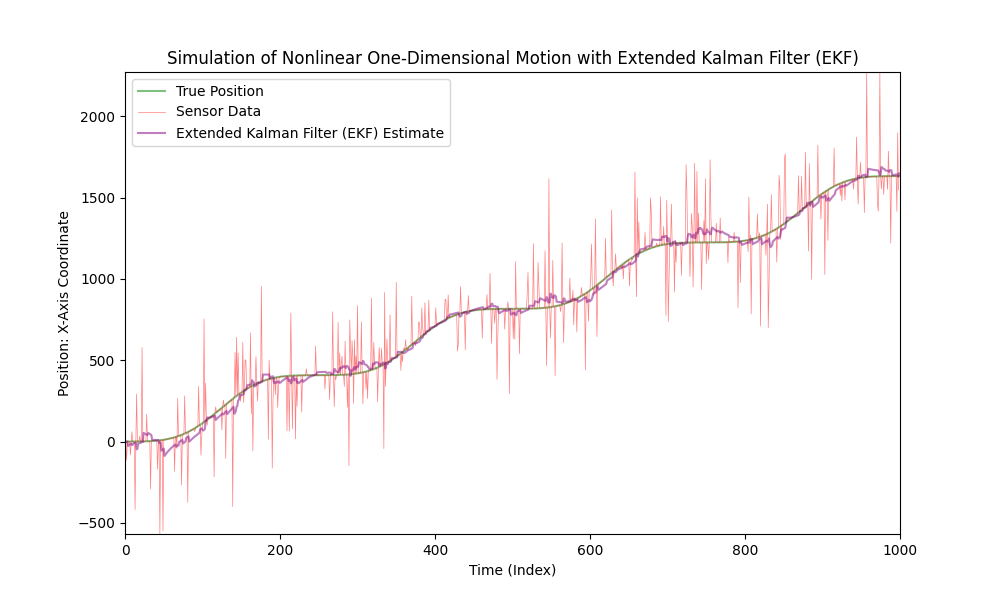
이제, 센서 노이즈의 수준을 크게 높여 봅시다.

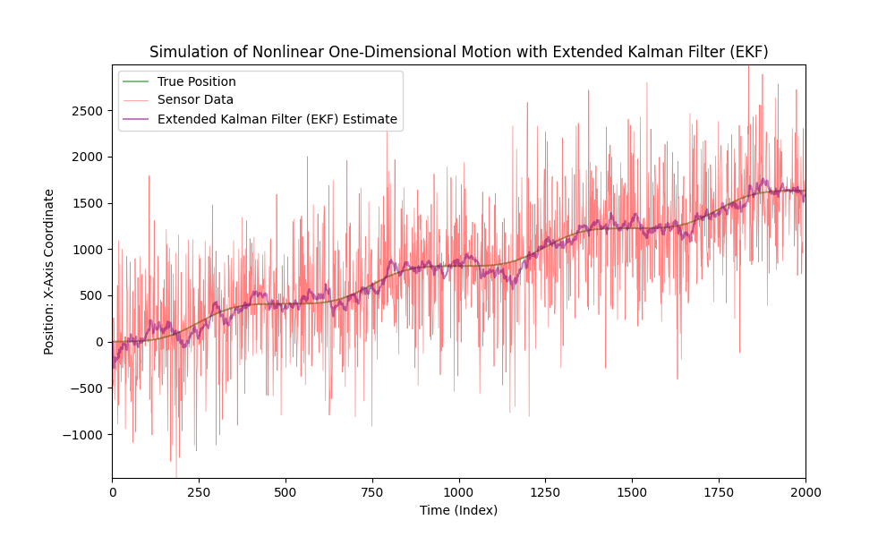
보시다시피, Extended Kalman Filter는 매우 잡음이 많은 데이터의 경우에도 잘 작동합니다.

추가 자료

https://en.wikipedia.org/wiki/Kalman_filter - 필터의 설명 및 그 기본적인 수학적 원리에 대한 설명.

https://kalmanfilter.org/cpp/index.html - C++에서 필터의 설명 및 구현.

https://commons.apache.org/proper/commons-math/javadocs/api-3.6.1/org/apache/commons/math3/filter/KalmanFilter.html - Java에서 필터의 설명 및 구현.

https://filterpy.readthedocs.io/en/latest/kalman/KalmanFilter.html - 필터의 설명 및 Python에서의 구현

결론

확장 칼만 필터(Extended Kalman Filter, EKF)는 동적 시스템의 상태를 추정하는 데 강력한 도구입니다, 특히 이 추정이 여러 센서의 데이터를 동시에 기반으로 할 필요가 있을 때에요. EKF의 주요 장점 중 하나는 다양한 출처의 정보를 통합할 수 있는 능력으로, 자동차 내비게이션 시스템, 로보틱스 또는 항공우주 공학과 같은 복잡한 시스템에서 매우 유용합니다.

다양한 센서에서 발생하는 소음이 많고 종종 불완전한 데이터를 고려할 때, EKF는 이 데이터를 통합하여 하나의 통일된 전체로 병합할 수 있는 능력이 있습니다. 정확하고 신뢰성 있는 상태 추정을 제공합니다. 예를 들어, 자동차에서 EKF는 GPS 데이터를 사용하여 위치를 결정하고 가속도계 데이터를 사용하여 속도와 가속도를 계산함으로써 차량의 움직임에 대한 보다 완전한 그림을 만들어낼 수 있습니다.

확장 칼만 필터(Extended Kalman Filter, EKF)는 각각의 센서에서 발생하는 노이즈와 오류로 인한 전체 불확실성을 줄일 수 있습니다. 이러한 오류들은 종종 상관관계가 없기 때문에, EKF에서의 공동 처리는 더욱 안정적이고 정확한 추정을 가능하게 합니다. 또한 EKF는 높은 강건성을 나타냅니다: 센서 중 하나에서 문제가 발생하는 경우, 시스템은 남은 센서들의 데이터에 의존하여 계속 작동할 수 있습니다. 이는 EKF를 신뢰성과 정확성이 매우 중요한 중요한 응용 분야에서 특히 가치있게 만듭니다. 다중 센서를 사용할 때 중요한 또 다른 측면은 측정의 시간 동기화입니다. EKF는 이러한 시간 차이를 능숙하게 처리하여 올바른 데이터 융합을 보장합니다.

EKF가 여러 소스에서 정보를 집계하고 분석할 수 있는 능력 덕분에 불확실성과 동적 변화가 있는 조건에서 고정밀 상태 추정이 필요한 분야에서 매우 소중한 도구입니다.

결론적으로, 센서 노이즈를 대응하는 소프트웨어는 정적, 통계적 방법들과 노이즈 유형 분류 및 완화를 위한 인공지능의 적용을 포함하는 도전적인 과정입니다.

저희 회사는 센서 노이즈 문제를 다루는 데 상당한 전문성을 보유하고 있습니다.

이 기사에 대해 문의하시고 싶으시면 언제든지 articles@stofu.io로 연락 주세요.

협력 기회에 대해 문의하시려면 info@stofu.io을(를) 통해 연락해 주세요.

우리의 저장소에서 모든 코드 파일을 찾을 수 있습니다: https://github.com/SToFU-Systems/EKF_Usage

모든 일이 잘 되길 바랍니다,

SToFU 시스템 팀

https://stofu.io

ADAS 센서 노이즈 처리를 위한 소프트웨어 접근 (1부)

ADAS란 무엇인가?

ADAS에서의 센서 노이즈

일차원 좌표 시스템에서의 점 움직임 시뮬레이션

칼만 필터

확장 칼만 필터 (Extended Kalman Filter, EKF)

추가 자료

결론

카테고리

최근 뉴스

ADAS 센서 노이즈 처리를 위한 소프트웨어 접근 (1부)

C++에서 PE 리소스 파서 (네이티브)

런스트를 이용한 윈도우 커널 개발 소개 (1부)

GPU 프로그래밍 소개

블랙매터 내부: 블랙매터 랜섬웨어의 기술적 분석