ADASセンサーのノイズ対応のソフトウェアアプローチ（パート1）

ADASとは何ですか？

現代の自動車は、ADAS（Advanced Driver Assistance Systems）のおかげでますます賢くなっており、道路の安全性を高め、運転を快適にしています。これらのシステムは、カメラ、レーダー、その他のセンサーを使用して車両の制御を支援し、他の車両、歩行者、信号機を検出し、道路状況や周囲の環境についての最新情報をドライバーに提供します。

ADASには、前方の交通に合わせて車の速度を調整するアダプティブクルーズコントロール、車を車線内に保つためのレーン管理システム、衝突を防ぐための自動ブレーキ、駐車操作を容易にするための自動駐車システムなど、さまざまな機能が含まれています。カメラ、レーダー、ライダー、超音波センサーなど、様々なタイプのセンサーがこれらのシステムの機能を確保し、車が道路状況やドライバーの運転スタイルに適応するのを助けます。

ADASのセンサーノイズ

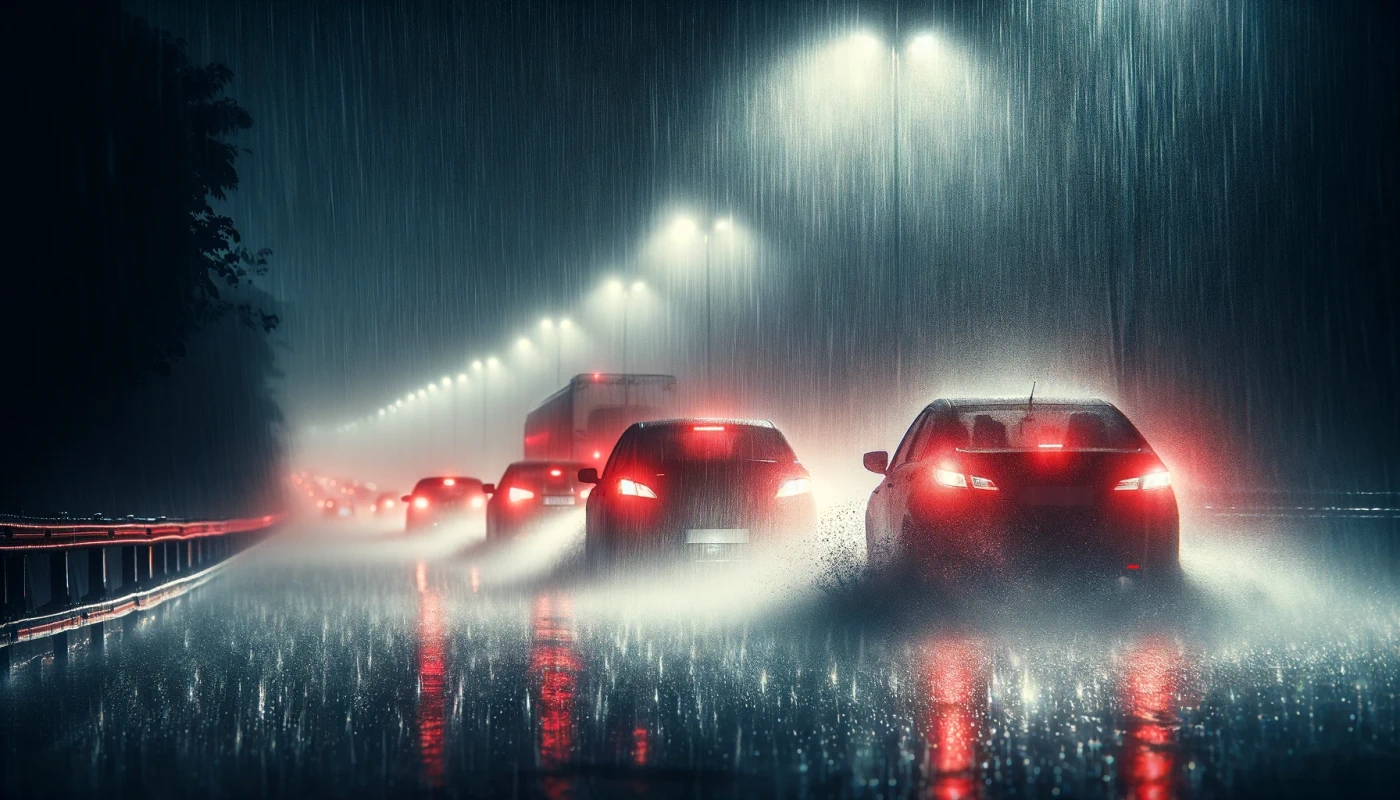
ADASセンサーは、その最新性や複雑さにも関わらず、ノイズの干渉を受けやすいです。これにはいくつかの理由があります。まず第一に、環境がセンサーに予測不可能な影響を及ぼすことがあります。たとえば、汚れ、ほこり、雨、雪がカメラやレーダーを覆い、受け取る情報が歪められることがあります。これは、汚れたガラスを通して物を見るようなものです：全てが見えないわけではありませんが、クリアではなく、多くのアーティファクトによって視界が遮られます。次に、センサー自体の技術的な制限もまたノイズの原因となることがあります。例えば、センサーは低照度条件や強い光のコントラストで性能が低下することがあります。これは、暗闇で何かを識別しようとすることや、非常に明るい光源を見ることに似ています―どちらの場合でも、細部を見ることが非常に困難になります。センサーから受け取ったデータが歪んだ場合、運転支援システムが道路状況を誤解することがあり、特定の状況では交通事故のリスクが高まる可能性があります。

一次元座標系における点の動きのシミュレーション

まず、一次元空間での車の動きをシミュレートするコードを書きましょう。このコードを実行するには、Python環境を設定し、必要なライブラリをインストールする必要があります。

ライブラリをインストールしてコードを実行する手順は以下の通りです：

コードを実行するには、Python環境をセットアップし、必要なライブラリをインストールする必要があります。以下にライブラリのインストールとコードの実行手順を示します：Pythonのインストール：もしPythonがまだない場合、公式のPythonウェブサイト（https://www.python.org/downloads/）からダウンロードしてインストールしてください。Pythonのバージョン3.xの使用を推奨します。
必要なライブラリをインストールする：コマンドラインを開き（WindowsではコマンドプロンプトまたはPowerShellになることがあります）、以下のコマンドを実行してライブラリをインストールします：
```
pip install matplotlib numpy filterpy
```
コードを保存する：提供されたコードをコピーして、拡張子が.pyのファイルに保存します（例：simulation.py
コードを実行する：コマンドラインで、コードファイルがあるディレクトリにナビゲートし、以下のコマンドで実行します：
```
python simulation.py 20 20 500
```
このコマンドは、ノイズの振幅に20、ノイズの頻度に20、グラフのデータ点の総数に500をそれぞれ用いてコードを実行します。必要に応じて引数の値を変更できます。

#
#  Copyright (C) 2024, SToFU Systems S.L.
#  All rights reserved.
#
#  This program is free software; you can redistribute it and/or modify
#  it under the terms of the GNU General Public License as published by
#  the Free Software Foundation; either version 3 of the License, or
#  (at your option) any later version.
#
#  This program is distributed in the hope that it will be useful,
#  but WITHOUT ANY WARRANTY; without even the implied warranty of
#  MERCHANTABILITY or FITNESS FOR A PARTICULAR PURPOSE.  See the
#  GNU General Public License for more details.
#
#  You should have received a copy of the GNU General Public License along
#  with this program; if not, write to the Free Software Foundation, Inc.,
#  51 Franklin Street, Fifth Floor, Boston, MA 02110-1301 USA.
#

import matplotlib.pyplot as plt
import numpy as np
from matplotlib.animation import FuncAnimation
import sys
import random
import time

# Named constants
AMPLITUDE_FACTOR = 5.0  # Factor for amplitude in the nonlinear acceleration function
WAVES = 4  # Number of waves in the nonlinear motion model
INITIAL_POSITION = 0  # Initial position
TRUE_VELOCITY_INITIAL = 2.0  # Initial true velocity (changed to float)
TRUE_VELOCITY_INCREMENT = 0.2  # Increment for true velocity (added as a constant)
PREDICTION_INTERVAL = 10  # Interval for predictions
DIM_X = 2  # Dimension of state vector in Kalman filter
DIM_Z = 1  # Dimension of measurement vector in Kalman filter
INITIAL_P_COVARIANCE = 1000  # Initial state covariance for Kalman filter
RANDOM_SEED = 42  # Seed for random number generator

# Initialize random number generator with the current time
random.seed(int(time.time()))  # Using the current time to initialize the random number generator

# Read noise_percentage, noise_probability, and total_points from command line arguments
noise_percentage = float(sys.argv[1]) / 100.0 if len(sys.argv) > 1 else 0.1
noise_probability = float(sys.argv[2]) / 100.0 if len(sys.argv) > 2 else 0.2
total_points = int(sys.argv[3]) if len(sys.argv) > 3 else 2000
interval = PREDICTION_INTERVAL / total_points  # Time interval between data points

# Define a nonlinear acceleration function that varies with time
def nonlinear_acceleration(t):
    # Calculate the amplitude of acceleration based on time
    amplitude = AMPLITUDE_FACTOR * 200.0 * (1 - abs((t % (total_points / WAVES) - (total_points / (2 * WAVES))) / (total_points / (2 * WAVES))))
    # Calculate the nonlinear acceleration based on time and amplitude
    return amplitude * np.sin(2.0 * np.pi * t / (total_points / WAVES))

# Function to add noise to true positions with a given probability
def add_noise(true_positions, probability):
    # Add Gaussian noise to true positions with specified probability
    return [p + np.random.normal(0, scale=noise_percentage * np.mean(true_positions)) if random.uniform(0, 1) <= probability else p for p in true_positions]

# Function to close the animation on pressing the ESC key
def close_animation(event):
    if event.key == 'escape':
        plt.close()

# Function for creating an animation without the Kalman Filter
def animate_without_ekf(i):
    plt.cla()
    # Plot the true position and sensor data up to the current time
    plt.plot(true_positions_nonlinear[:i], color='green', alpha=0.5, label='True Position')
    plt.plot(sensor_positions_with_noise[:i], color='red', alpha=0.5, label='Sensor Data', linewidth=0.5)

    # Set plot limits and labels
    plt.xlim(0, total_points)
    plt.ylim(min(true_positions_nonlinear + sensor_positions_with_noise),
             max(true_positions_nonlinear + sensor_positions_with_noise))
    plt.xlabel('Time (Index)')
    plt.ylabel('Position: X-Axis Coordinate')
    plt.title('Simulation of Nonlinear One-Dimensional Motion')

    # Display the legend
    plt.legend()

# Main entry point of the code
if __name__ == "__main__":
    # Create a figure for the animation
    fig, ax = plt.subplots(figsize=(10, 6))

    # Use connect to add an event handler for key presses
    fig.canvas.mpl_connect('key_press_event', close_animation)

    # Initialize true_positions_nonlinear with the initial position and true_velocity
    true_positions_nonlinear = [INITIAL_POSITION]
    true_velocity = TRUE_VELOCITY_INITIAL

    # Generate true positions based on the nonlinear motion model
    for t in range(1, total_points):
        acc = nonlinear_acceleration(t)
        true_velocity += acc * interval
        true_positions_nonlinear.append(true_positions_nonlinear[-1] + true_velocity * interval)

    # Add noise to true positions to simulate sensor data
    sensor_positions_with_noise = add_noise(true_positions_nonlinear, noise_probability)

    # Create the animation using FuncAnimation
    ani = FuncAnimation(fig, animate_without_ekf, frames=total_points, interval=interval * 1000, repeat=False)

    # Display the animation
    plt.show()

これは一次元空間での車の動きのシミュレーションです：

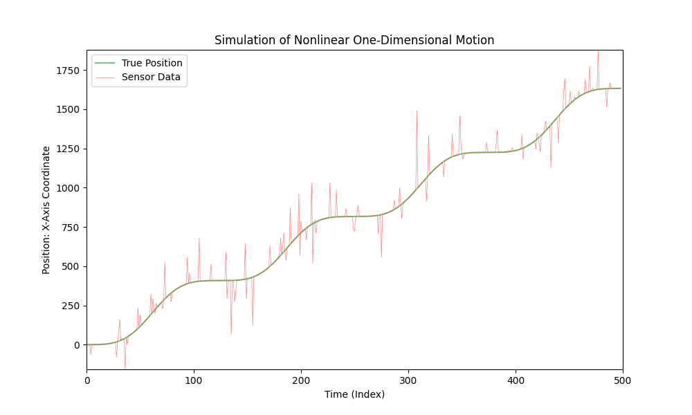
車は変化する加速度で移動し、センサーが車のX座標を測定します。このシミュレーションでは、可能な測定誤差を考慮してセンサーデータにノイズを加えます。

先に提供されたコードはこのシミュレーションを視覚化しており、緑の線は車の「真の」位置を表し、赤の線は追加されたノイズを考慮したセンサーデータを表しています。加速度は時間とともに変化し、車の動きのより現実的なシミュレーションを作り出しています。

このコードは、変化する加速度と可能なセンサーエラーを考慮して、車の動きのさまざまなシナリオを視覚化し分析するために使用できます。

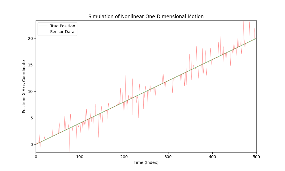
直線運動をシミュレートするには、nonlinear_acceleration(t) 関数を常に0を返すように単純に修正できます：

def nonlinear_acceleration(t):
    return 0

この変更により、車の動きが一定の速度で直線的になります。

カルマンフィルタ

Kalman Filter（カルマンフィルタ）は、1960年にRudolf E. Kalmanによって開発されたアルゴリズムです。このアルゴリズムは、不完全でノイズのある測定値のセットに基づいて動的システムの状態を推定することを可能にします。初期には、カルマンフィルターは航空宇宙工学の問題に対処するために開発されましたが、時間が経つにつれて、さまざまな分野で広く応用されています。カルマンフィルターの主な利点は、再帰的であることです。つまり、最新の測定値と前の状態を使用してシステムの現在の状態を計算します。これにより、オンラインでのリアルタイムデータ処理に効率的です。

Kalman Filterは、ナビゲーションや車両制御、シグナル処理、計量経済学、ロボティクスなど多岐にわたる分野で応用されており、不完全または不完全なデータに基づいて時間変動プロセスを推定する必要がある多くの他の領域でも使用されています。

Kalman Filterは、他のデータ推定およびフィルタリングアルゴリズムに対していくつかの重要な利点があります:

最適性：特定の条件（線形システム、ガウスノイズ）の下で、カルマンフィルタは平均二乗推定誤差を最小限に抑える点で最適です。
リアルタイム効率: カルマンフィルタは再帰的であり、最新の測定値と前の状態のみを使用して現在の状態を計算します。これにより、リアルタイムアプリケーションに適しています。
最小メモリ要件: フィルタは最新の測定と現在の状態推定のみを使用するため、データの全履歴を保存する必要がありません。
測定誤差への強さ: フィルタはノイズの多いデータを効率的に処理する能力があり、ランダムな測定誤差の影響を最小限に抑えます。
多様な応用: その汎用性のため、カルマンフィルタは航空宇宙工学から計量経済学まで、多様な分野で応用されています。
実装の容易さ: アルゴリズムは比較的理解しやすく、実装も容易であるため、幅広い専門家にアクセス可能です。

センサーが騒がしい測定値で一定の速度で動く一次元システムの中で私たちの車の位置を測定するセンサー用の基本的なカルマンフィルターを実装しましょう。

#
#  Copyright (C) 2024, SToFU Systems S.L.
#  All rights reserved.
#
#  This program is free software; you can redistribute it and/or modify
#  it under the terms of the GNU General Public License as published by
#  the Free Software Foundation; either version 3 of the License, or
#  (at your option) any later version.
#
#  This program is distributed in the hope that it will be useful,
#  but WITHOUT ANY WARRANTY; without even the implied warranty of
#  MERCHANTABILITY or FITNESS FOR A PARTICULAR PURPOSE.  See the
#  GNU General Public License for more details.
#
#  You should have received a copy of the GNU General Public License along
#  with this program; if not, write to the Free Software Foundation, Inc.,
#  51 Franklin Street, Fifth Floor, Boston, MA 02110-1301 USA.
#

import matplotlib.pyplot as plt
import numpy as np
from matplotlib.animation import FuncAnimation
from filterpy.kalman import KalmanFilter
from filterpy.common import Q_discrete_white_noise
import sys
import random

# Read noise_percentage, noise_probability, total_points from the command line
noise_percentage = float(sys.argv[1]) / 100.0 if len(sys.argv) > 1 else 0.1
noise_probability = float(sys.argv[2]) / 100.0 if len(sys.argv) > 2 else 0.2
total_points = int(sys.argv[3]) if len(sys.argv) > 3 else 2000
interval = 10 / total_points

# Initialize true positions and velocity
true_positions_linear = [0]
true_velocity = 2

for t in range(1, total_points):
    true_positions_linear.append(true_positions_linear[-1] + true_velocity * interval)

# Function to add noise to true positions
def add_noise(true_positions, probability):
    return [p + np.random.normal(0, scale=noise_percentage * np.mean(true_positions))
            if random.uniform(0, 1) <= probability else p for p in true_positions]

sensor_positions_with_noise = add_noise(true_positions_linear, noise_probability)

# Initialize Kalman Filter (KF)
kf = KalmanFilter(dim_x=2, dim_z=1)
kf.F = np.array([[1, interval],
                 [0, 1]])
kf.H = np.array([[1, 0]])
kf.P *= 1000
kf.R = noise_percentage * np.mean(true_positions_linear)
kf.Q = Q_discrete_white_noise(dim=2, dt=interval, var=0.001)

x = np.array([[sensor_positions_with_noise[0]],
              [0]])
kf_positions = [x[0, 0]]

# Function to update Kalman Filter with sensor data
def update_kalman_filter(z):
    kf.predict()
    kf.update(z)
    return kf.x[0, 0]

# Function to create an animation with Kalman Filter (KF) estimation
def animate_with_kalman(i):
    plt.cla()
    plt.plot(true_positions_linear[:i], color='green', alpha=0.5, label='True Position')
    plt.plot(sensor_positions_with_noise[:i], color='red', alpha=0.5, linewidth=0.5, label='Sensor Data')

    if i < total_points:
        kf_estimate = update_kalman_filter(sensor_positions_with_noise[i])
        kf_positions.append(kf_estimate)

    plt.plot(kf_positions[:i + 1], color='blue', alpha=0.5, label='Kalman Filter (KF) Estimate')

    plt.xlim(0, total_points)
    plt.ylim(min(true_positions_linear + sensor_positions_with_noise),
             max(true_positions_linear + sensor_positions_with_noise))
    plt.xlabel('Time (Index)')
    plt.ylabel('Position: X-Axis Coordinate')
    plt.title('Simulation of Linear One-Dimensional Motion with Kalman Filter (KF)')
    plt.legend()

# Main entry point
if __name__ == "__main__":
    # Create a figure and animation
    fig, ax = plt.subplots(figsize=(10, 6))
    ani = FuncAnimation(fig, animate_with_kalman, frames=total_points, interval=interval * 1000, repeat=False)

    # Display the animation
    plt.show()

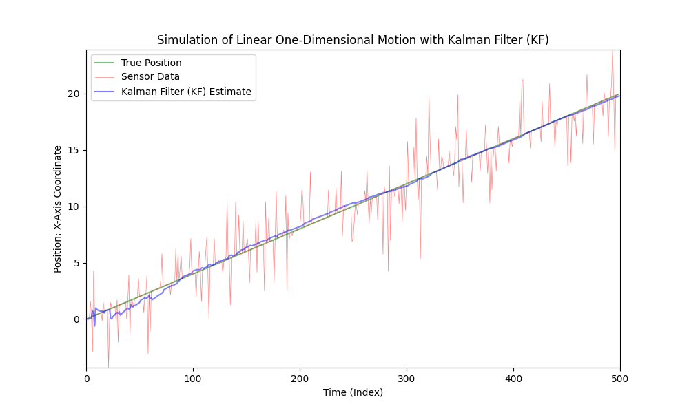
ご覧のとおり、カルマンフィルタは強いノイズがある線形システムに適しています。しかし、車の動きは線形ではありません。車はさまざまな大きさと方向で加速します。

コードを少し複雑にして、車の動きを非線形にし、可変加速度を導入しましょう。シンプルさと明瞭さのために、加速度をモデル化するのに正弦関数を使用します。ノイズレベルは同じままに保ちます。

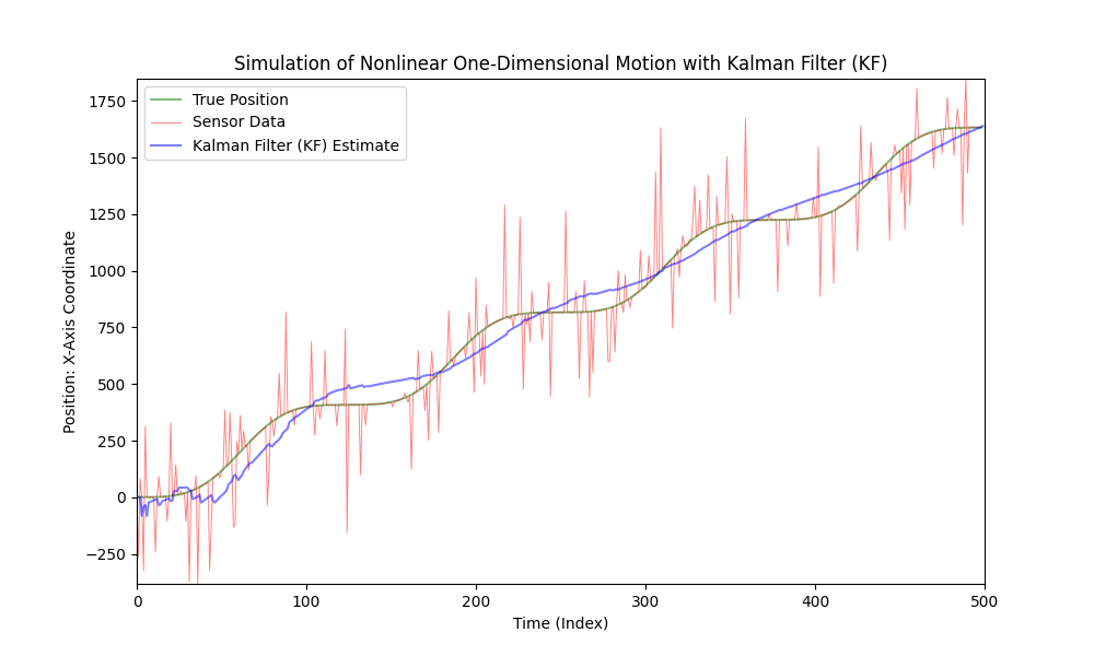
ご覧のとおり、古典的なカルマンフィルターは非線形モデルには適していません。そのために、拡張カルマンフィルター（EKF）が開発されました。

拡張カルマンフィルタ (EKF)

拡張カルマンフィルタ（EKF）は、非線形システムに対応するために設計された古典的なカルマンフィルタの改良版です。標準的なカルマンフィルタが線形システム用に設計されているのに対し、EKFは非線形の場合に対応するようにその適用範囲を拡張します。

Extended Kalman Filterは、元々のKalman Filterが1960年にRudolf Kalmanによって導入された後に開発されました。それは、1960年代と1970年代に、航空宇宙および海洋航行分野においてKalman Filterを非線形システムに適応させるため、エンジニアや科学者による取り組みの結果として出現しました。その創造の正確な日付や具体的な作者はあまり知られていませんが、EKFは徐々に進化し、さまざまな研究グループの枠組みの中で発展しました。

拡張カルマンフィルタ（EKF）は、非線形方程式で記述されたシステムの状態推定が必要なタスクで広く使用されています。主な応用分野には、ロボティクス（ロボットの位置と向きの推定）、自動車産業（自動運転システムやナビゲーションにおいて）、航空宇宙工学（衛星軌道ナビゲーションや宇宙船）、モバイル通信、その他多くの技術や工学の分野が含まれます。

Extended Kalman Filter (EKF)と標準Kalman Filterの主な違いは、システムのダイナミクスと測定をどのように扱うかにあります。

主な違いは以下の通りです：

非線形の取り扱い：標準的なカルマンフィルターは、システムのダイナミクスと測定プロセスが線形であると仮定します。これは、状態遷移および測定機能が線形行列として表現できることを意味します。拡張カルマンフィルター（EKF）は、非線形システムに対応するように設計されています。線形行列の代わりに、非線形関数を使用してシステムダイナミクスおよび測定プロセスを記述します。
線形化：EKFでは、現在の状態推定値の周りでの一次テーラー級数展開を通じて、非線形関数を近似するために線形化が使用されます。これにより、状態遷移および測定機能の線形化された対応物が提供され、フィルターで使用されます。
状態遷移および測定機能：標準カルマンフィルターでは、状態遷移および測定機能は行列（例えば、状態遷移行列および測定行列）によって表現されます。EKFでは、これらの機能は任意の微分可能な非線形関数であることができます。これにより柔軟性が増しますが、複雑さと計算要件も増加します。
計算の複雑さ：EKFは、非線形関数を線形化する必要性とその後の計算により、より高い計算複雑性を必要とします。

拡張カルマンフィルターと標準カルマンフィルターの主な違いは、非線形関数とその線形化を使用して非線形システムで動作する能力にあります。

#
#  Copyright (C) 2024, SToFU Systems S.L.
#  All rights reserved.
#
#  This program is free software; you can redistribute it and/or modify
#  it under the terms of the GNU General Public License as published by
#  the Free Software Foundation; either version 3 of the License, or
#  (at your option) any later version.
#
#  This program is distributed in the hope that it will be useful,
#  but WITHOUT ANY WARRANTY; without even the implied warranty of
#  MERCHANTABILITY or FITNESS FOR A PARTICULAR PURPOSE.  See the
#  GNU General Public License for more details.
#
#  You should have received a copy of the GNU General Public License along
#  with this program; if not, write to the Free Software Foundation, Inc.,
#  51 Franklin Street, Fifth Floor, Boston, MA 02110-1301 USA.
#

import matplotlib.pyplot as plt
import numpy as np
from matplotlib.animation import FuncAnimation
from filterpy.kalman import KalmanFilter
from filterpy.common import Q_discrete_white_noise
import sys
import random

# Named constants
AMPLITUDE_FACTOR = 5.0  # Factor for amplitude in the nonlinear acceleration function
WAVES = 4  # Number of waves in the nonlinear motion model
INITIAL_POSITION = 0  # Initial position
TRUE_VELOCITY_INITIAL = 2.0  # Initial true velocity (changed to float)
TRUE_VELOCITY_INCREMENT = 0.2  # Increment for true velocity (added as a constant)
PREDICTION_INTERVAL = 10  # Interval for predictions
DIM_X = 2  # Dimension of state vector in Kalman filter
DIM_Z = 1  # Dimension of measurement vector in Kalman filter
INITIAL_P_COVARIANCE = 1000  # Initial state covariance for Kalman filter

# Initialize random number generator with the current time
random.seed()

# Read noise_percentage, noise_probability, and total_points from command line arguments
noise_percentage = float(sys.argv[1]) / 100.0 if len(sys.argv) > 1 else 0.1
noise_probability = float(sys.argv[2]) / 100.0 if len(sys.argv) > 2 else 0.2
total_points = int(sys.argv[3]) if len(sys.argv) > 3 else 2000
interval = PREDICTION_INTERVAL / total_points  # Time interval between data points

# Define a nonlinear acceleration function that varies with time
def nonlinear_acceleration(t):
    # Calculate the amplitude of acceleration based on time
    amplitude = AMPLITUDE_FACTOR * 200.0 * (1 - abs((t % (total_points / WAVES) - (total_points / (2 * WAVES))) / (total_points / (2 * WAVES))))
    # Calculate the nonlinear acceleration based on time and amplitude
    return amplitude * np.sin(2.0 * np.pi * t / (total_points / WAVES))

# Function to add noise to true positions with a given probability
def add_noise(true_positions, probability):
    # Add Gaussian noise to true positions with specified probability
    return [p + np.random.normal(0, scale=noise_percentage * np.mean(true_positions)) if random.uniform(0, 1) <= probability else p for p in true_positions]

# Function to update the Extended Kalman Filter (EKF) with sensor measurements
def update_extended_kalman_filter(z):
    ekf.predict()  # Predict the next state
    ekf.update(z)  # Update the state based on sensor measurements
    return ekf.x[0, 0]  # Return the estimated position

# Функция для закрытия анимации при нажатии клавиши ESC
def close_animation(event):
    if event.key == 'escape':
        plt.close()

# Function for creating an animation with EKF estimates
def animate_with_ekf(i):
    plt.cla()
    # Plot the true position and sensor data up to the current time
    plt.plot(true_positions_nonlinear[:i], color='green', alpha=0.5, label='True Position')
    plt.plot(sensor_positions_with_noise[:i], color='red', alpha=0.5, label='Sensor Data', linewidth=0.5)

    if i < total_points:
        # Update the EKF with the current sensor measurement and obtain the estimate
        ekf_estimate = update_extended_kalman_filter(sensor_positions_with_noise[i])
        ekf_positions.append(ekf_estimate)

    # Plot the EKF estimate up to the current time
    plt.plot(ekf_positions[:i + 1], color='purple', alpha=0.5, label='Extended Kalman Filter (EKF) Estimate')

    # Set plot limits and labels
    plt.xlim(0, total_points)
    plt.ylim(min(true_positions_nonlinear + sensor_positions_with_noise),
             max(true_positions_nonlinear + sensor_positions_with_noise))
    plt.xlabel('Time (Index)')
    plt.ylabel('Position: X-Axis Coordinate')
    plt.title('Simulation of Nonlinear One-Dimensional Motion with Extended Kalman Filter (EKF)')
    plt.legend()

# Main entry point of the code
if __name__ == "__main__":
    # Create a figure for the animation
    fig, ax = plt.subplots(figsize=(10, 6))

    # Используйте connect для добавления обработчика событий
    fig.canvas.mpl_connect('key_press_event', close_animation)

    # Initialize true_positions_nonlinear with the initial position and true_velocity
    true_positions_nonlinear = [INITIAL_POSITION]
    true_velocity = TRUE_VELOCITY_INITIAL

    # Generate true positions based on the nonlinear motion model
    for t in range(1, total_points):
        acc = nonlinear_acceleration(t)
        true_velocity += acc * interval
        true_positions_nonlinear.append(true_positions_nonlinear[-1] + true_velocity * interval)

    # Add noise to true positions to simulate sensor data
    sensor_positions_with_noise = add_noise(true_positions_nonlinear, noise_probability)

    # Initialize an Extended Kalman Filter (EKF)
    ekf = KalmanFilter(dim_x=DIM_X, dim_z=DIM_Z)
    ekf.F = np.array([[1, interval],
                    [0, 1]])
    ekf.H = np.array([[1, 0]])
    ekf.P *= INITIAL_P_COVARIANCE
    ekf.R = noise_percentage * np.mean(true_positions_nonlinear)

    ekf_x = np.array([[sensor_positions_with_noise[0]],
                    [0]])
    ekf_positions = [ekf_x[0, 0]]

    # Create the animation using FuncAnimation
    ani = FuncAnimation(fig, animate_with_ekf, frames=total_points, interval=interval * 1000, repeat=False)

    # Display the animation
    plt.show()

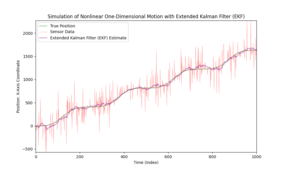
非線形運動に拡張カルマンフィルタを適用します。

それでは、センサーノイズのレベルを大幅に上げてみましょう。

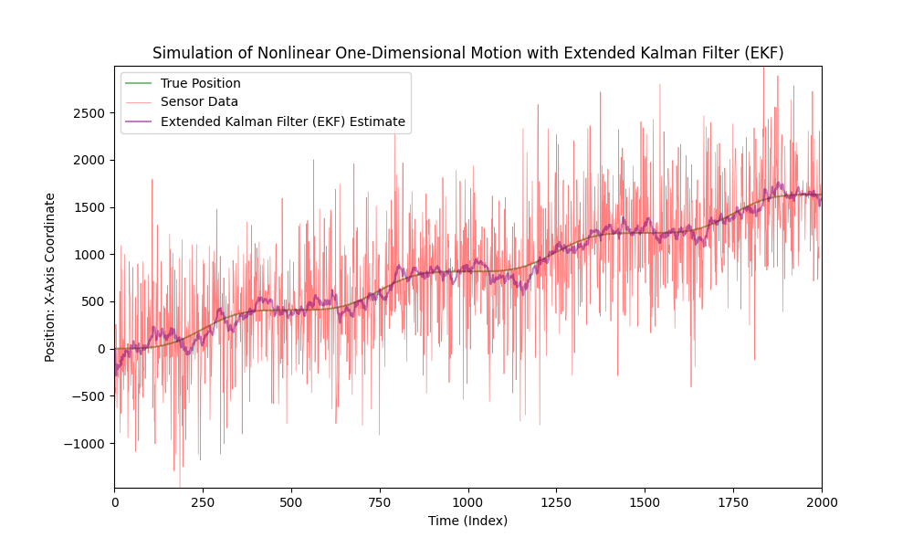
ご覧のとおり、Extended Kalman Filterは非常にノイズの多いデータの場合でもうまく機能します。

追加資料

https://en.wikipedia.org/wiki/Kalman_filter - フィルターの説明およびその基本的な数学的原理について。

https://kalmanfilter.org/cpp/index.html - C++でのフィルターの説明と実装。

https://commons.apache.org/proper/commons-math/javadocs/api-3.6.1/org/apache/commons/math3/filter/KalmanFilter.html - フィルターの説明とJavaでの実装。

https://filterpy.readthedocs.io/en/latest/kalman/KalmanFilter.html - Pythonでのフィルターの説明と実装

結論

拡張カルマンフィルタ（EKF）は、特にこの推定が複数のセンサーからのデータに基づいて行う必要がある場合に、動的システムの状態を推定するための強力なツールです。EKFの主な利点の一つは、様々な情報源からの情報を統合する能力にあり、これにより自動車のナビゲーションシステム、ロボティクス、または航空宇宙工学などの複雑なシステムで非常に便利です。

さまざまなセンサーからの騒がしく、しばしば不完全なデータを考慮して、EKFはこのデータを統合して一つの完全なものにすることが可能です。これにより、より正確で信頼性の高い状態推定を提供します。例えば、車内でEKFはGPSデータを使用して位置を特定し、加速度計のデータを利用して速度と加速度を計算することで、車の動きのより完全なイメージを作り出すことができます。

拡張カルマンフィルタ（EKF）は、各センサーのノイズやエラーに起因する全体的な不確実性を減少させる能力があります。これらのエラーはしばしば無相関であるため、EKFでの共同処理により、より安定して正確な見積もりが可能になります。また、EKFは非常に頑強であることも注目に値します。センサーの1つに問題が発生した場合でも、システムは残りのデータに依存して動作を続けることができます。これにより、信頼性と精度が最も重要なクリティカルなアプリケーションでEKFが特に価値あるものとなっています。複数のセンサーを使用する際のもう一つの重要な側面は、計測の時間同期です。EKFはこれらの時間差を巧みに扱い、正確なデータ融合を保証します。

複数の情報源から情報を集約し分析する能力のおかげで、EKFは不確実性や動的変化の条件下で高精度な状態推定が求められる分野において、非常に価値のあるツールです。

結論として、センサーノイズと戦うソフトウェアは、静的、統計的方法と人工知能を用いたノイズタイプの分類及び軽減の適用を含む、難しいプロセスです。

弊社はセンサーノイズの問題を扱うためのかなりの専門知識を持っています。

この記事に関するお問い合わせは、お気軽に以下のアドレスまでご連絡ください articles@stofu.io。

コラボレーションの機会については、info@stofu.ioまでお問い合わせください。

すべてのコードファイルは私たちのリポジトリで見つけることができます: https://github.com/SToFU-Systems/EKF_Usage

皆さんに最善を願っています。

SToFUシステムズチーム

https://stofu.io

ADASセンサーのノイズ対応のソフトウェアアプローチ（パート1）

ADASとは何ですか？

ADASのセンサーノイズ

一次元座標系における点の動きのシミュレーション

カルマンフィルタ

拡張カルマンフィルタ (EKF)

追加資料

結論

カテゴリー

最近のニュース

ADASセンサーのノイズ対応のソフトウェアアプローチ（パート1）

C++でのPEリソースパーサー（ネイティブ）

RustでのWindowsカーネル開発入門（パート1）

GPUプログラミング入門

BlackMatter内部：BlackMatterランサムウェアの技術解析